Continuous Cholesky Factorization

This note was inspired by the plenary talk by Joel A. Tropp at SIAM LA24. While I could not find the specific talk online a very similar talk was recorded at the Boeing Colloquium Series. In the talk Joel presented the work of ^[1], and I will in this note make the relation between that work and that on continuous matrix factorizations by Alex Townsend ^[2].

The (discrete) Cholesky factorization

The Cholesky factorization of a positive semidefinite matrix \(\mathbf{K}\) is given by

\[ \mathbf{K} = \mathbf{L}\mathbf{L}^\top \in \mathbb{R}^{n\times n}, \]

where \(\mathbf{L}\) is a lower triangular matrix. Where \(\mathbf{L}\) and \(\mathbf{L}^\top\) are the factors of interest. The factorization is useful as it can be used to solve the linear systems \(\mathbf{K}\mathbf{s} =\mathbf{t}\) by performing two triangular solves (\(\mathbf{L}\mathbf{y} = \mathbf{t}, \mathbf{L}^\top\mathbf{s} = \mathbf{y}\)). The Cholesky factorization can be computed by performing \(n\) rank-1-updates of the original matrix. The first iterate is

\[ \mathbf{K}^{(0)} = \begin{bmatrix}k & \mathbf{m}^\top \\ \mathbf{m} & \mathbf{M}\end{bmatrix} = \frac{1}{k}\begin{bmatrix}k \\ \mathbf{m}\end{bmatrix}\begin{bmatrix}k \\ \mathbf{m}\end{bmatrix}^\top + \underbrace{\begin{bmatrix} 0 & 0 \\0 & \mathbf{M} - \mathbf{m}\mathbf{m}^\top /k\end{bmatrix}}_{\text{Residual. Denoted by } \mathbf{K}^{(1)}}. \]

Each iteration eliminates a row and a column of the residual \(\mathbf{K}^{(i)}\), with the first residual being the matrix itself. Thus after \(r\) rank-1-update we have eliminated \(r\) rows and columns of \(\mathbf{K}\). The rows and columns that gets eliminated at the \(i\)th iteration is called the \(i\)th pivot. After \(n\) iterations every row and column have been eliminated and we have the full factorization.

In this note we will be mostly be interested in the partial Cholesky factorization, which corresponds to the Cholesky factorization after \(r\) iterations. The partial Cholesky factorization will be a rank \(r\) approximation of \(\mathbf{K}\). The aim is that if \(r \ll n\), then the approximation is a "data efficient" representation of \(\mathbf{K}\). There exist various of approaches of how to chose the pivots ^[2]

In ^[1] it is argued that the randomized approach works best. But why? In short it is stable with respect to the ordering of the data.

Kernel matrices and kernel functions

The motivation for the note is that of Gaussian process regression. A key concept in Gaussian process regression is that of a kernel matrix. The kernel matrix, \(\mathbf{K}\), is a matrix whose elements are generated from a so-called kernel function \(k(\mathbf{x},\mathbf{y})\).

\[ \mathbf{K}_{ij} = k(\mathbf{x}_i, \mathbf{x}_j),\ \text{ where }\ \mathbf{x}_i, \mathbf{x}_j \in X \]

where \(X = \{\mathbf{x}_1, \mathbf{x}_2, \dots, \mathbf{x}_n \}\) is a collection of data points. An important property of the kernel function is that it is positive semidefinite

\[ k(\mathbf{x},\mathbf{x}) \geq 0, \]

which has the consequence of the resulting kernel matrix \(\mathbf{K}\) is positive semidefinite. This is important since the kernel matrix represent the correlation between the the data points in \(X\). A commonly used kernel function is the squared exponential given by

\[ k(\mathbf{x},\mathbf{x}) = \exp\left(\frac{\|\mathbf{x}_i - \mathbf{x}_j\|_2^2}{2\ell}\right), \]

where \(\ell\) is commonly referred to as the length scale.

To illustrate the process we simulate data points \(\mathbf{x}_i \in [-2,2]\) and plot both the discrete / observed kernel matrix \(\mathbf{K}\) and the continuos kernel function. Two things to note: First that the \(y-\)axes below are flipped to conform to the standard kernel matrix form and secondly that the data is sorted, giving some structure to the kernel matrix.

using LinearAlgebra, StatsBase, Plots, Random, InvertedIndices
Random.seed!(1234)

n = 20  # Number of data points
k = 5   # Rank of approximation
dim = 1 # Dimension of data
l = 2.0 # Lengthscale parameter

X = [rand(floor(Int,n/3),dim) .- 2; rand(floor(Int,n/3),dim); rand(floor(Int,n/3),dim)/2 .+ 1.5] # Three groups
n = length(X) # Number of data points
X = sort(X[:]) # Soring the data - Not strictly necessary, but makes the discrete form nicer
G(x,y,l=l) = exp(-norm(x-y)^2/(2*l))

# The actual view is in 2D
o = ones(n)
Xx = kron(X,o)
Xy = kron(o,X)
Gk = [G(x,y) for (x,y) in zip(Xx,Xy)]
plot_matrix = heatmap(sort(X[:]),sort(X[:]),reshape(Gk,n,n),aspect_ratio=:equal, title="Discrete")
scatter!(plot_matrix,Xx,Xy, label=false)
xlabel!(plot_matrix,"x"); ylabel!(plot_matrix,"y"); yflip!(true)

Xc = range(-2,2,300)
plot_smooth = contour(Xc,Xc, (x,y) -> G(x,y), fill=true,aspect_ratio=:equal,clim=(0,1))
xlabel!(plot_smooth,"x"); ylabel!(plot_smooth,"y"); yflip!(true)
scatter!(plot_smooth,Xx,Xy, label=false,title="Continuous")
scatter!(plot_smooth,X,X, label=false, color=:black)
plot(plot_matrix,plot_smooth, layour=(1,2),dpi=300)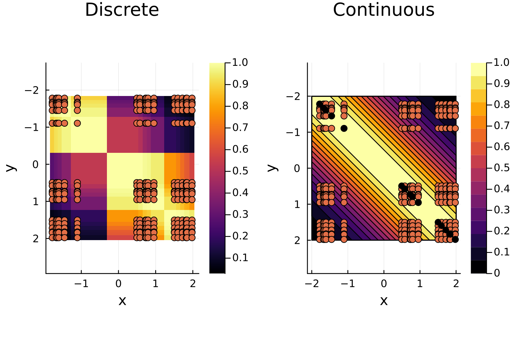

The continuous Cholesky factorization

Approximating the discrete form with a low-rank matrix is as easy performing a partial Cholesky. However, a different approach is needed in order to approximate the continuous form the a "low-rank" function. In ^[2] continuous analogous to matrix factorization is introduced in the context of so-called cmatrices. These matrices can be represented as function of two continuous variables, i.e. that they are elements of \(C([a,b]\times[c,d])\). While the properties is only stated for scalar \(x\) and \(y\) one can easily extend the ideas for a general bivariate function such as a kernel function.

The continuous Cholesky factorization of rank \(r\) of kernel function is given as

\[ k(\mathbf{x},\mathbf{y}) \approx \sum_{i=1}^{r}\frac{k_i(\mathbf{x},\mathbf{x}_i)k_i(\mathbf{x}_i, \mathbf{y})}{k_i(\mathbf{x}_i, \mathbf{x}_i)} = \sum_{i=1}^{r}\frac{k_i(\mathbf{x},\mathbf{x}_i)}{\sqrt{k_i(\mathbf{x}_i, \mathbf{x}_i)}}\frac{k_i(\mathbf{x}_i, \mathbf{y})}{\sqrt{k_i(\mathbf{x}_i, \mathbf{x}_i)}} \]

where \((\mathbf{x}_i,\mathbf{x}_i)\) are the so-called pivot points and

\[ k_i(\mathbf{x},\mathbf{y}) = \begin{cases} k(\mathbf{x},\mathbf{y}) \quad &i = 1\\ k_{i-1}(\mathbf{x},\mathbf{y}) - \frac{k_{i-1}(\mathbf{x},\mathbf{x}_{i-1})k_{i-1}(\mathbf{x}_{i-1},\mathbf{y})}{k_{i-1}(\mathbf{x}_{i-1},\mathbf{x}_{i-1})}\quad &i \geq 2. \end{cases} \]

Note that \(k(\mathbf{x},\mathbf{x}_i)\) and \(k(\mathbf{x}_i,\mathbf{y})\) can be viewed as removing the columns and rows

Visual Representations

The Greedy Approach

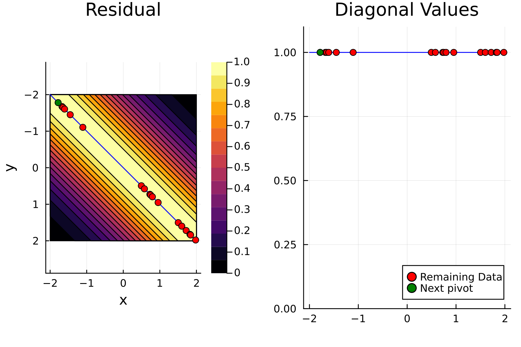
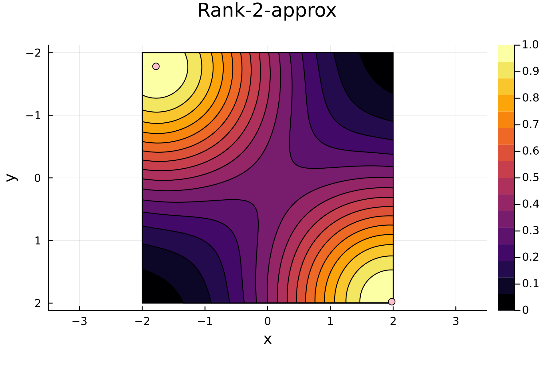
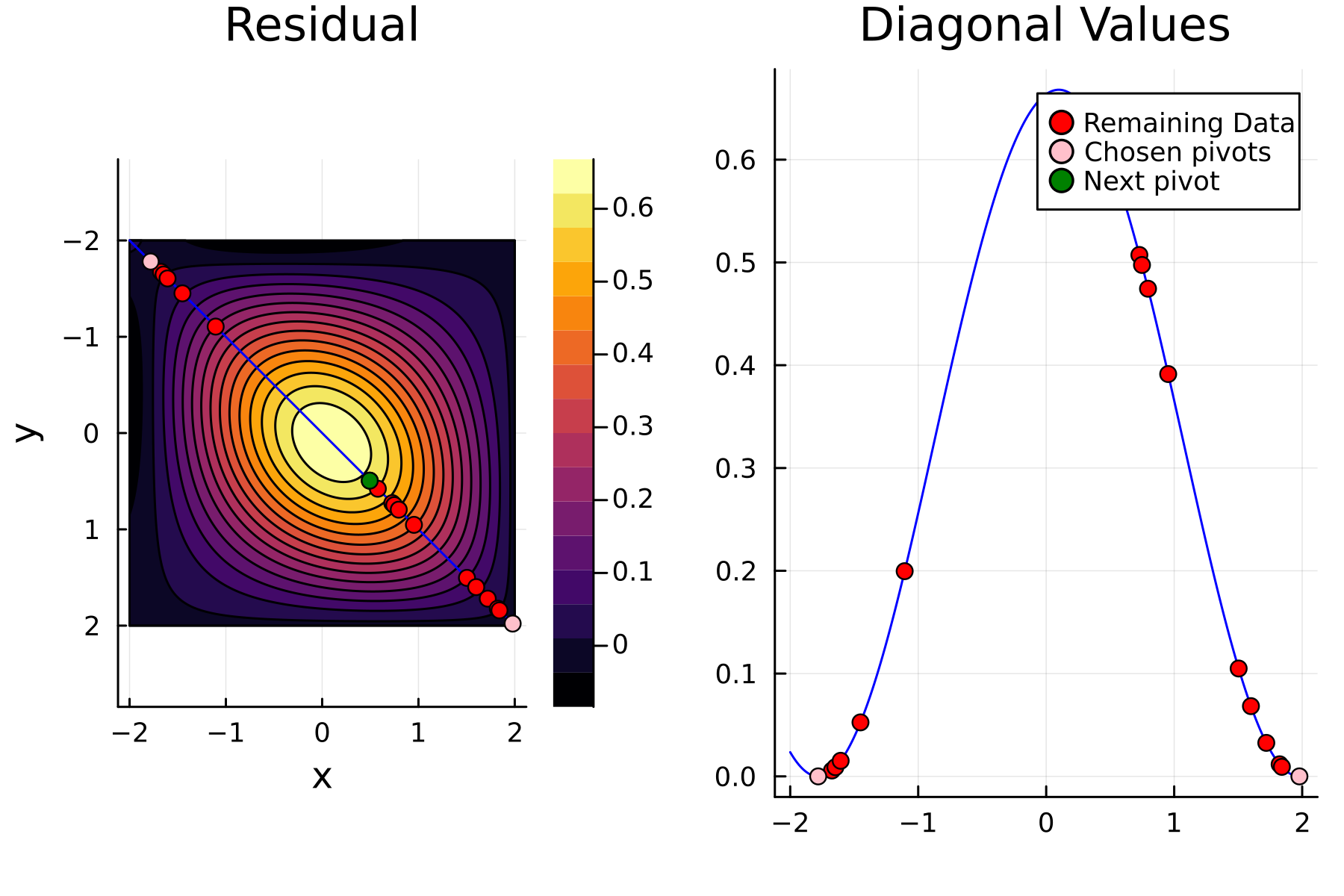
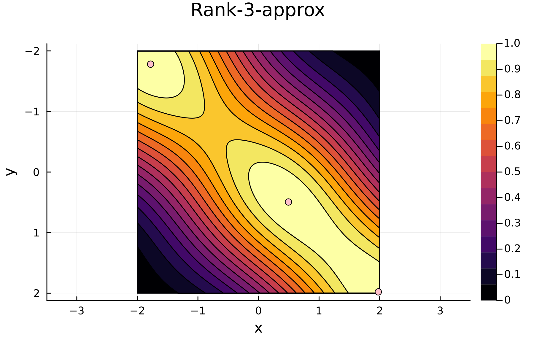
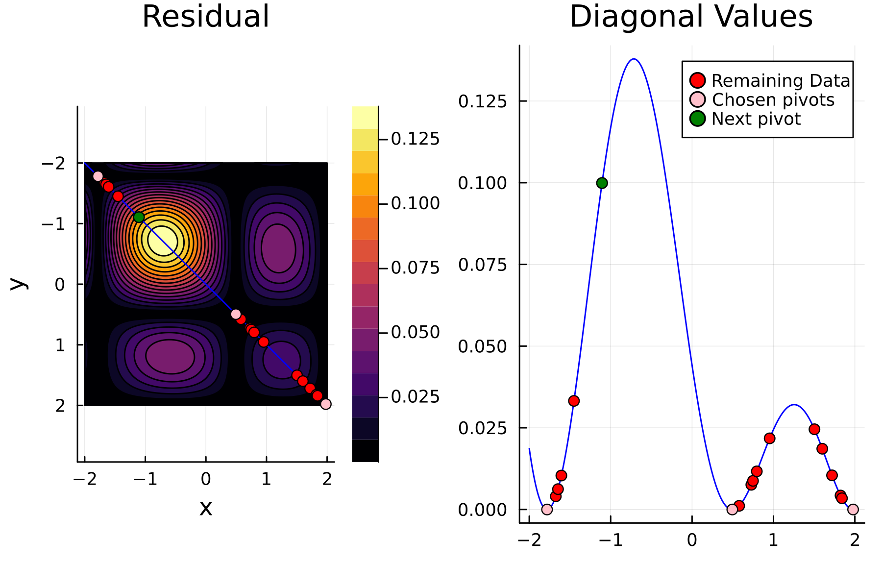
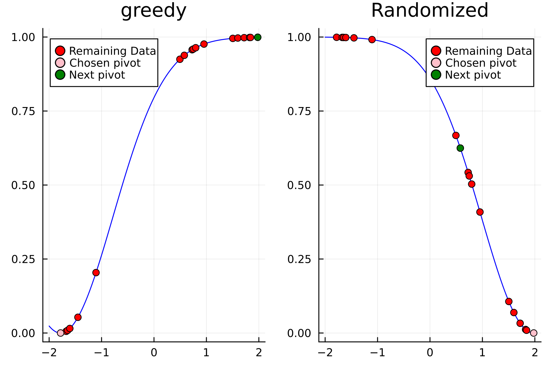
As the initial residual is just the matrix itself \((\mathbf{K}^{(0)})\) then its diagonal is filled with ones. As such the greedy method will simply pick the first pivot depending on the ordering of the data. This is one of the weaknesses of the greedy method, namely that is susceptible to bad ordering of the data. In fact ^[1] gives an example full of outliers. On this example the greedy approach completely fails and gets stuck picking the pivots equal to the ordering of the data. Note that had the ordering of the data in ^[1] been random, then implicitly the greedy method would not have failed.

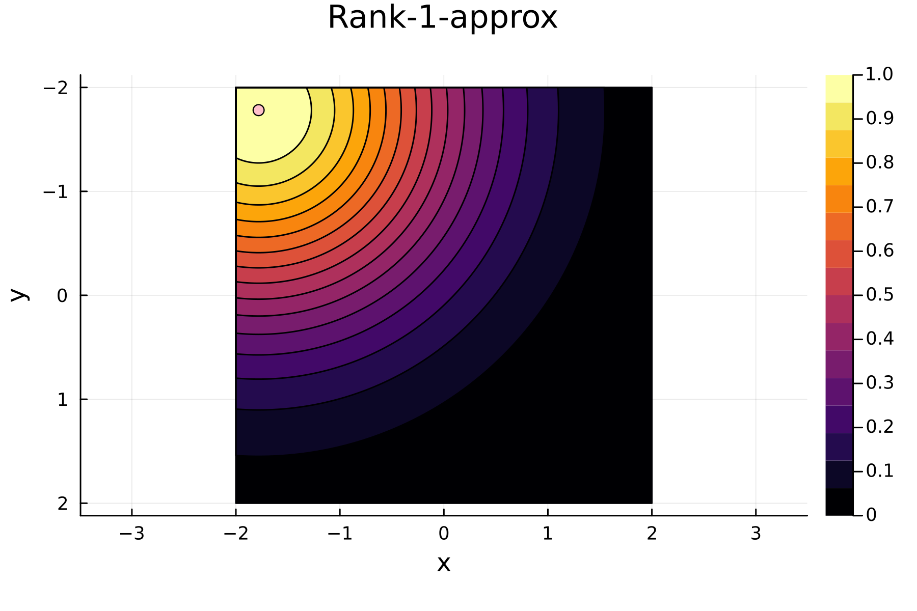
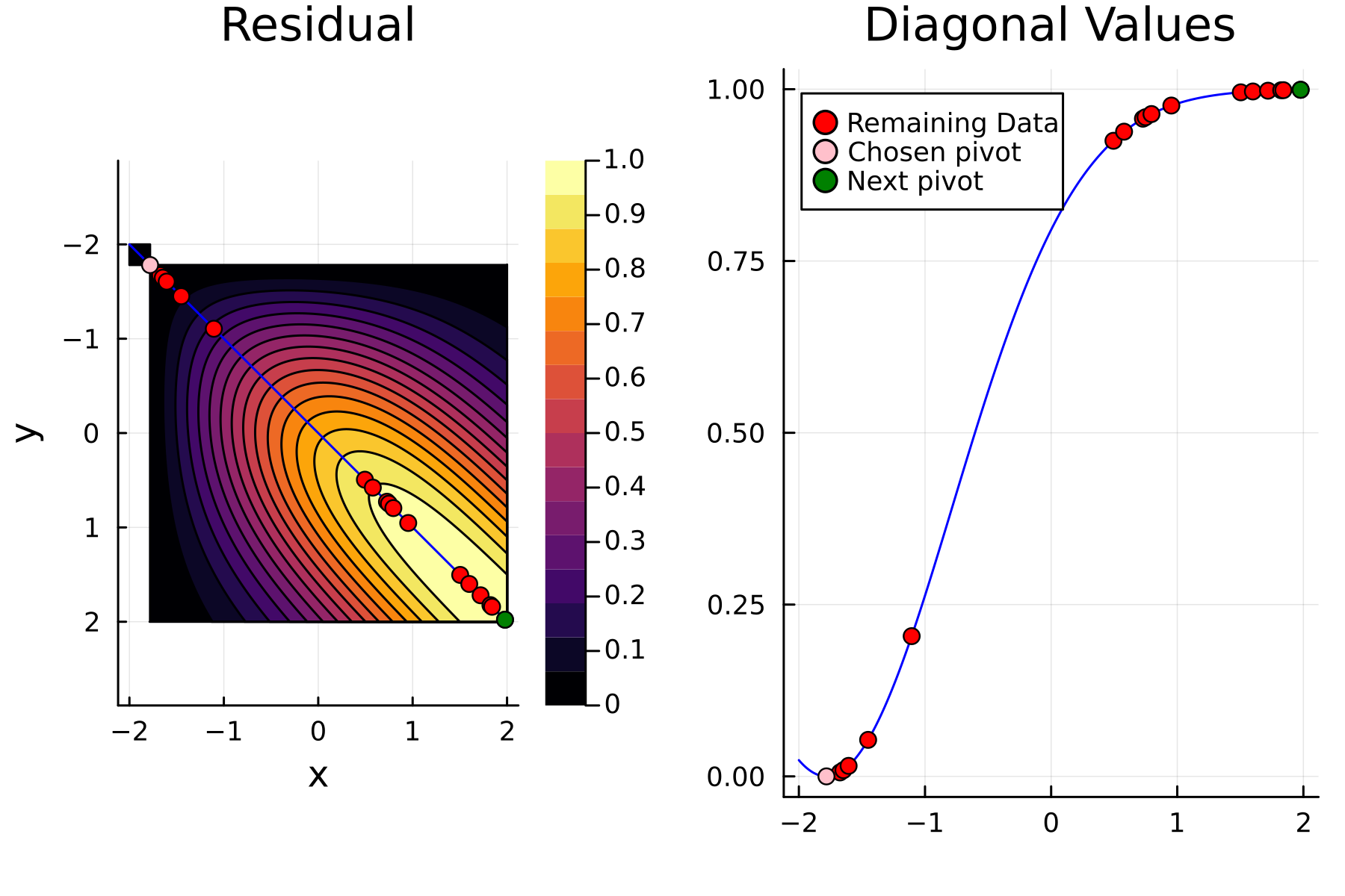
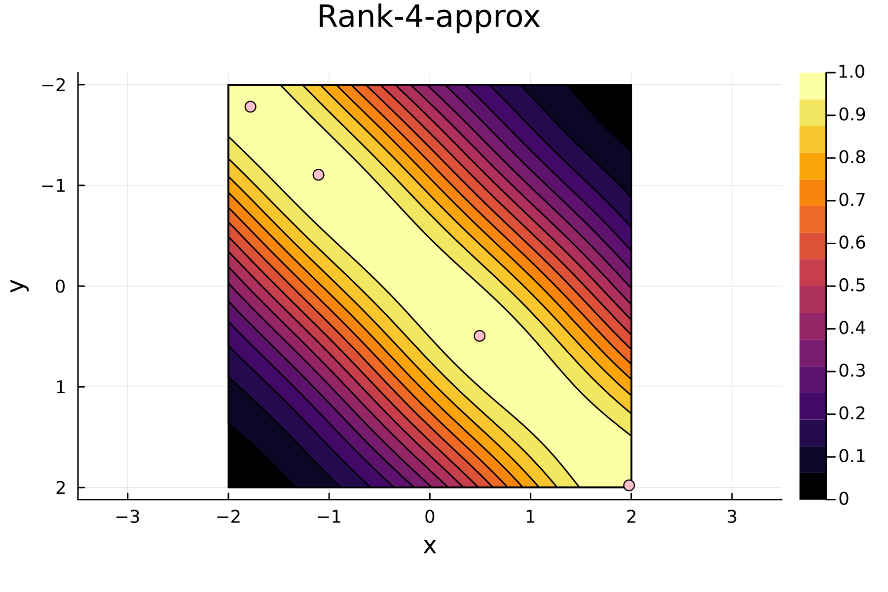
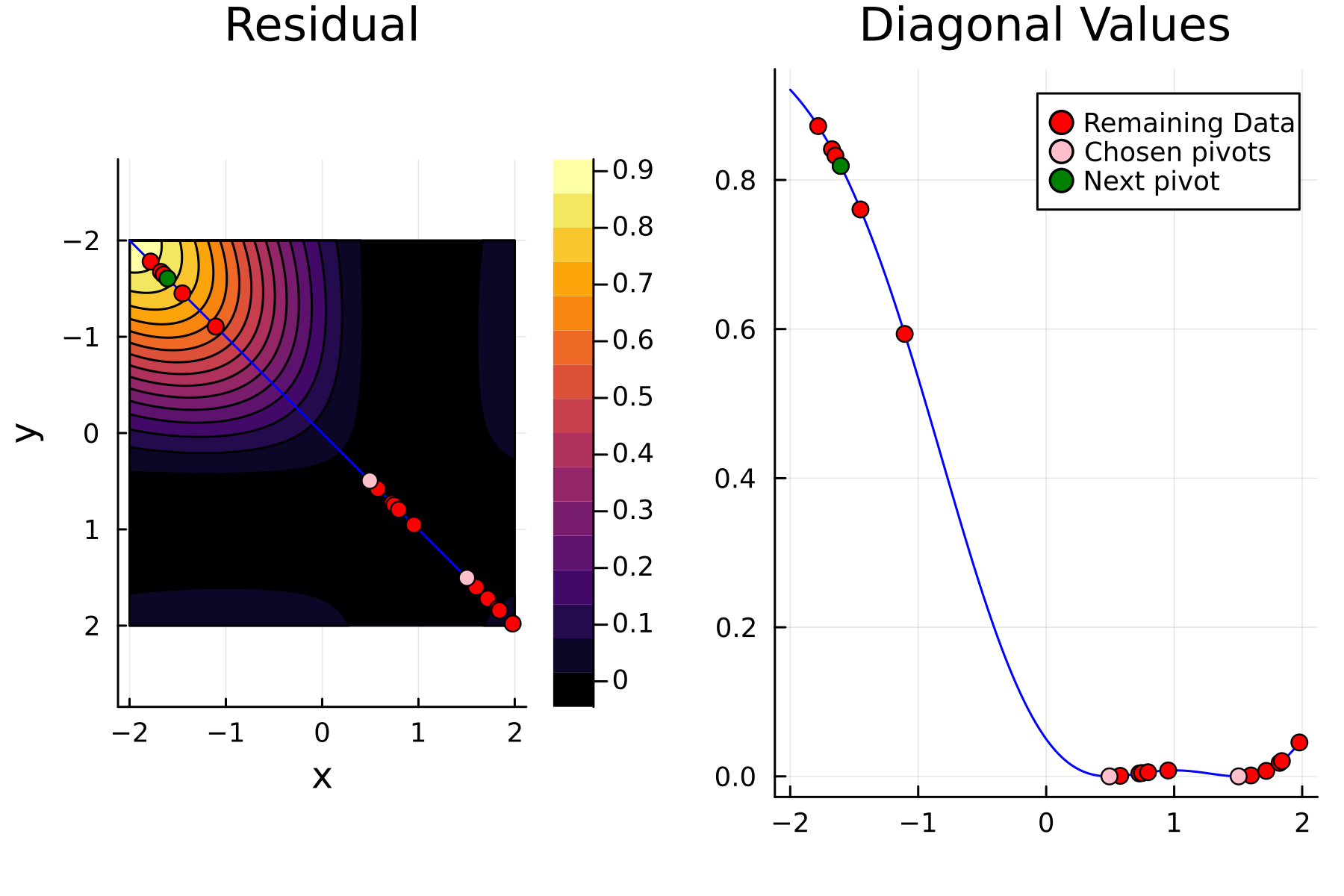
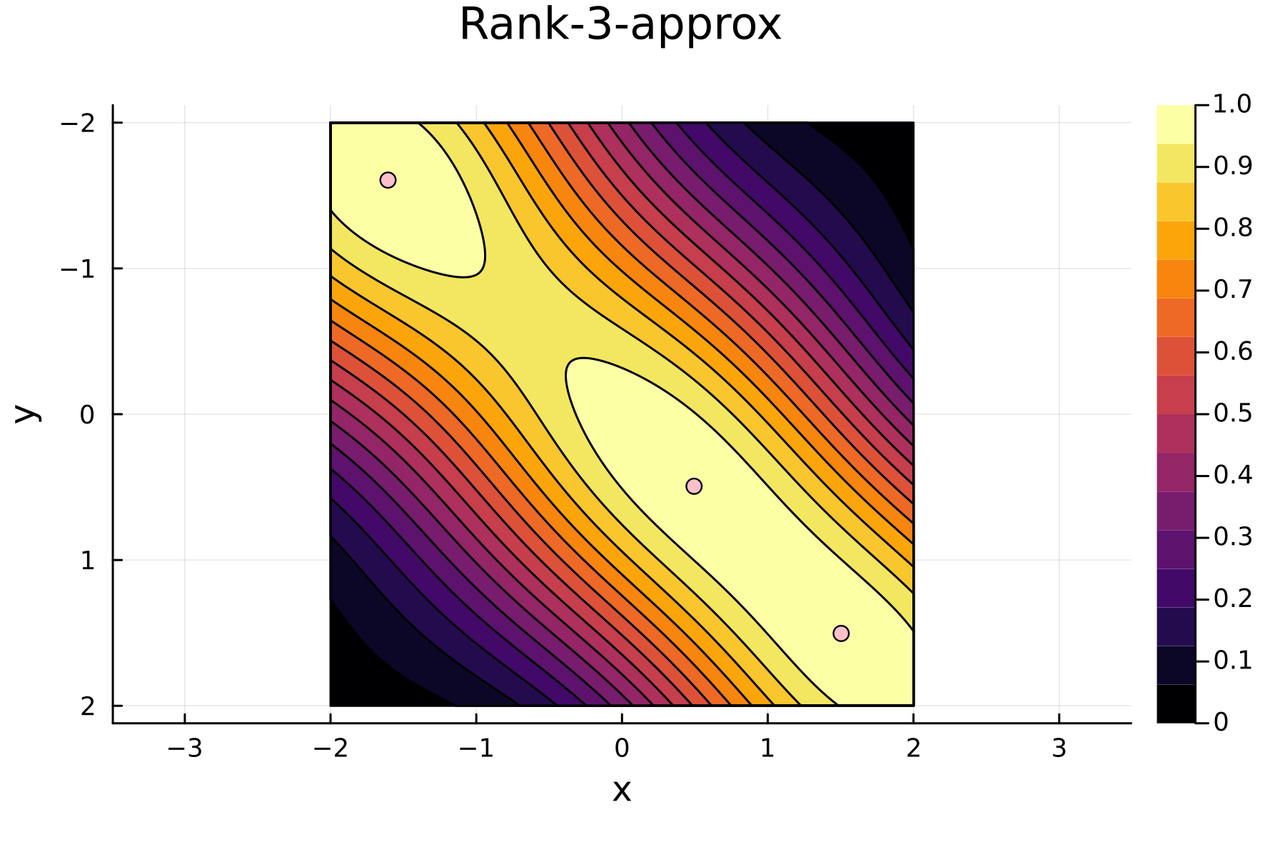
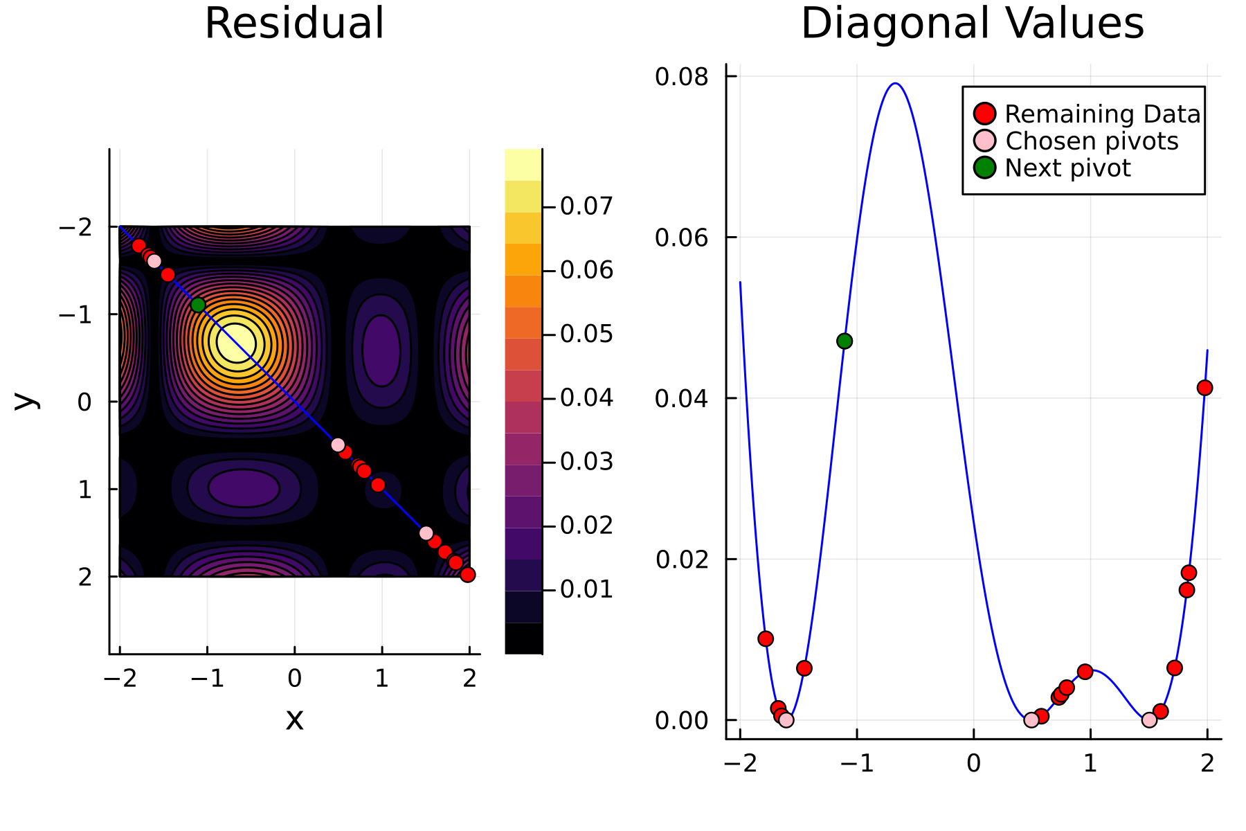
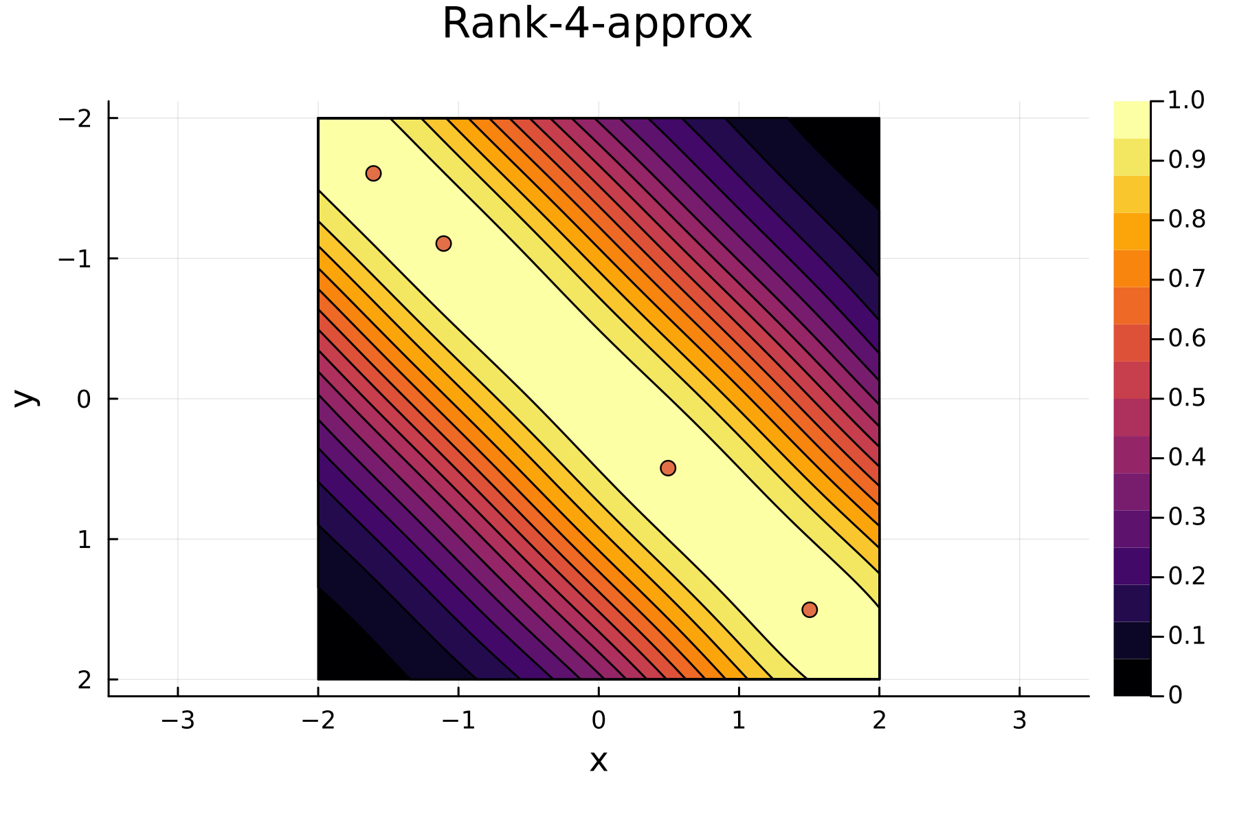
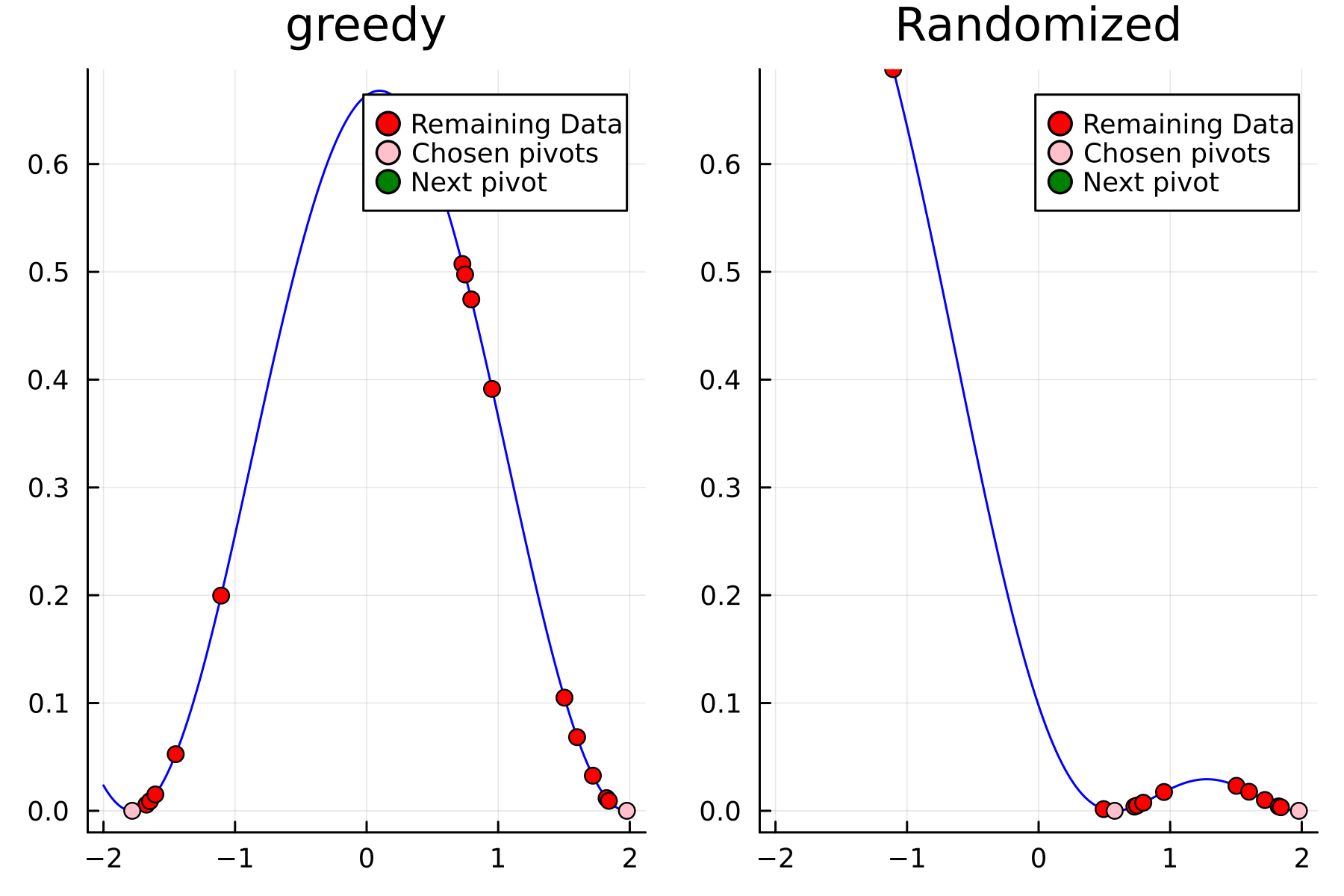
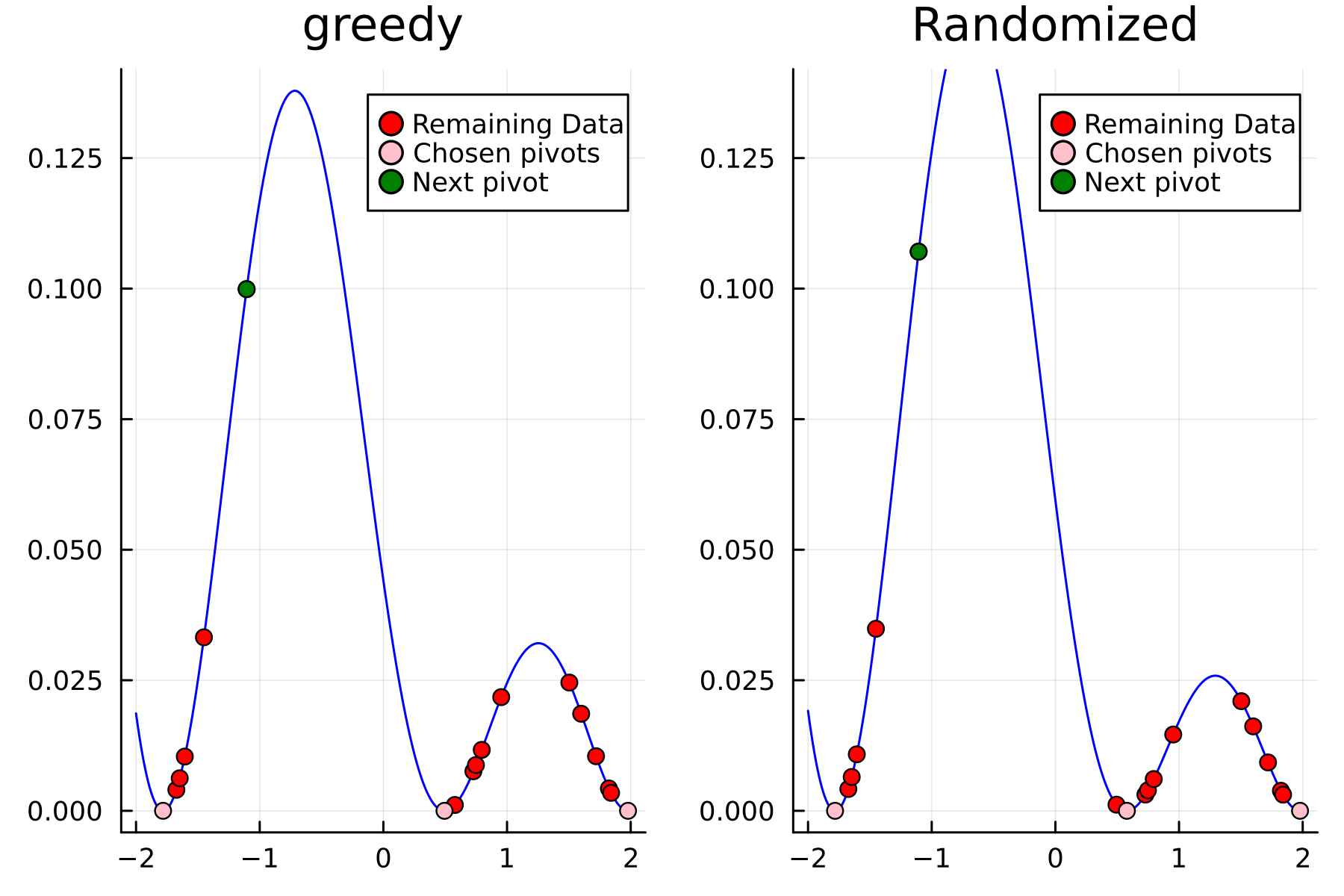
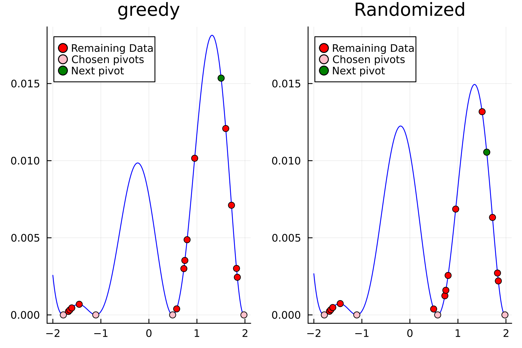
In the previously data introduces is completely ordered w.r.t. \(x\), and the greedy method therefore picks the first pivot as the point with smallest value. The next iteration again start by looking at the diagonal, but this time of the residual \(\mathbf{K}^{(1)}\). Given that the first pivot was chosen as smallest value, it is no surprise that the worst approximation happens furthest away. As such the next pivot point will be at the largest value. The two iterations highlight the weakness of the greedy method: In most cases it ends up picking pivots on the borders of the dataset.

The series of the first 4 iterations can be seen below.

1st iteration

2nd iteration

3rd iteration

4th iteration

The Randomized Approach

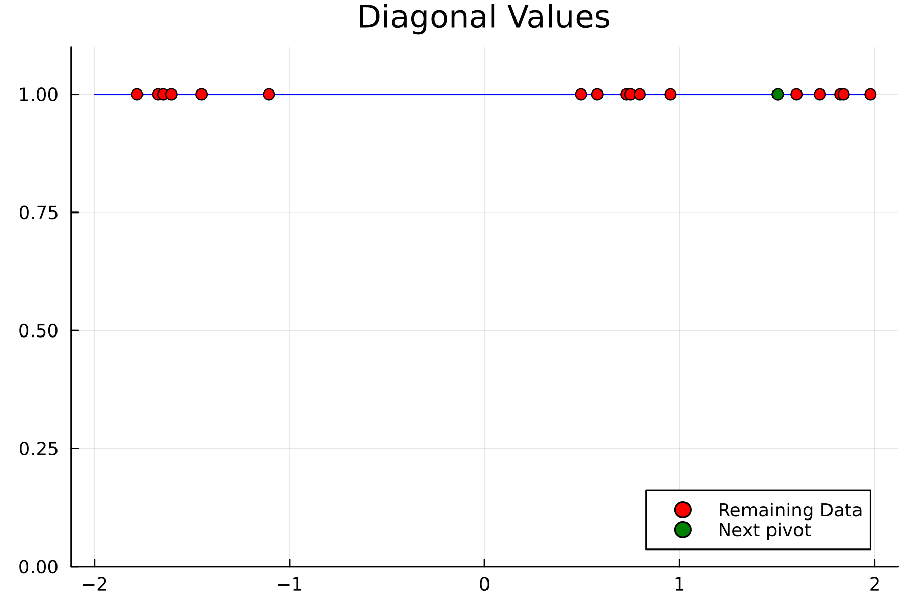
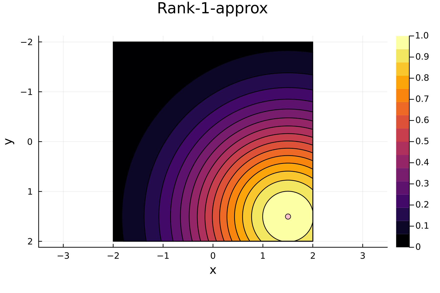
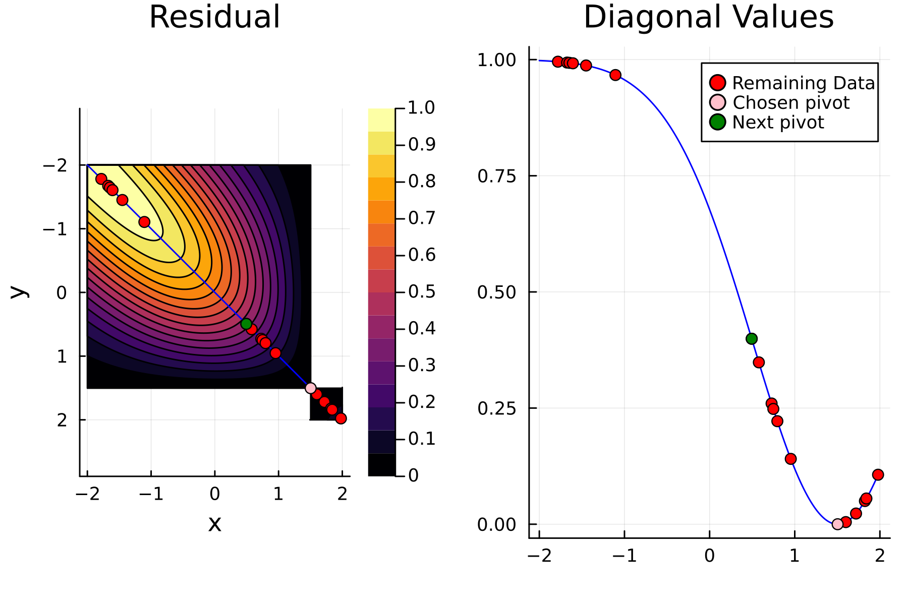
We now repeat the first 4th, but using randomized pivoting approach. A noticeable difference between the greedy and the randomized approach is that the randomized approach prioritizes (with some probability off course) to pick points close to where the data actually is. This is a win, as a point "inside" of the dataset will reduce the overall diagonal of the residual in the places of where data is actually located. In addition the approach is also completely robust against the ordering of the data, as a randomization of the data is built directly into the approach.

1st iteration

2nd iteration

3rd iteration

4th iteration

Comparing diagonals

To highlight the differences between the two approaches we plot the diagonals together. The overall decay of the diagonal is similar for each methods. However, the residual within the dataset is clearly smaller for the randomized approach as compared to the greedy approach. A downside of the randomized approach is that the approximation is not as good "outside" of the data. Said differently, the randomized approach generalizes worse than the greedy approach, by relying on pivots inside, rather than the border, of the dataset.

References

[1]	Chen, Y., Epperly, E., Tropp, J., & Webber, R. (2022). Randomly pivoted Cholesky: Practical approximation of a kernel matrix with few entry evaluations. arXiv e-prints, arXiv:2207.06503.

[2]	Townsend, A., & Trefethen, L. N. (2015). Continuous analogues of matrix factorizations. Proceedings of the Royal Society A: Mathematical, Physical and Engineering Sciences, 471(2173), 20140585. https://doi.org/10.1098/rspa.2014.0585