Thinking of "sparse plus low-rank" as a graph
A general matrix-plus-low-rank is given by
\[ A + UV^\top, \quad A \in \mathbb{R}^{n\times n},\ U,V \in \mathbb{n\times r} \]In the case of \(A\) being sparse (\(A\) is often diagonal - e.g. in Nesterov Todd scaling of a second-order cones), this matrix will structure. However, this structure will not be utilized if one e.g. naively solves the linear system
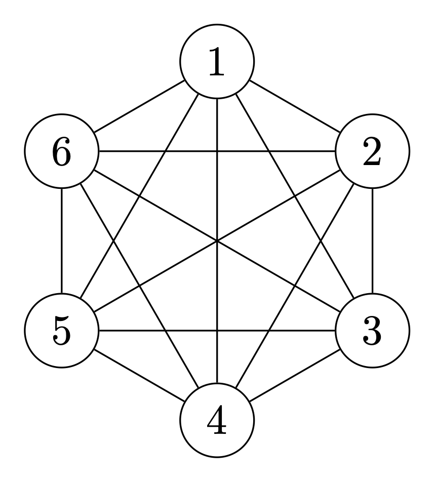
\[ \left(A + UV^\top\right)x = b, \]as forming the product \(UV^\top\) will result in a dense matrix. Thinking of a matrix as a graph, then a dense matrix can be represented as a connected graph. An example of connected graph representing a dense \(6\times6\) matrix can be seen below.

Computationally a connected graph is prohibitive, as it means that all nodes are communicating. Worse so adding an extra node will result in adding \(n\) edges. Furthermore, in the case of \(A\) being a sparse matrix we lose the sparsity when the connected graph of \(UV^\top\) is added. Thankfully, forming the product \(UV^\top\) can be circumvented by introducing an auxiliary variable \(\alpha\) so that
\[ Ax + U\left(\underbrace{V^\top x}_{\alpha}\right) = Ax + U\underbrace{\alpha}_{V^\top x} = b. \]By explicitly writing out the relation \(\alpha = V^\top x\) as \(V^\top x - \alpha = 0\) (so that the unknowns \(x\) and \(\alpha\) are on the same side) we get the following linear system
\[ \begin{bmatrix} A & U \\ V^\top & -I \end{bmatrix} \begin{bmatrix} x\\ \alpha \end{bmatrix} = \begin{bmatrix} b \\ 0 \end{bmatrix}. \]In the above system the sparsity of \(A\) can be utilized, with the cost of adding the low-rank term being the addition of dense rows (\(V^\top\)) and columns \((U)\) and a diagonal matrix \(-I\). For even modestly sized matrices the above representation comes with a significant reduction in memory usage and computational time.
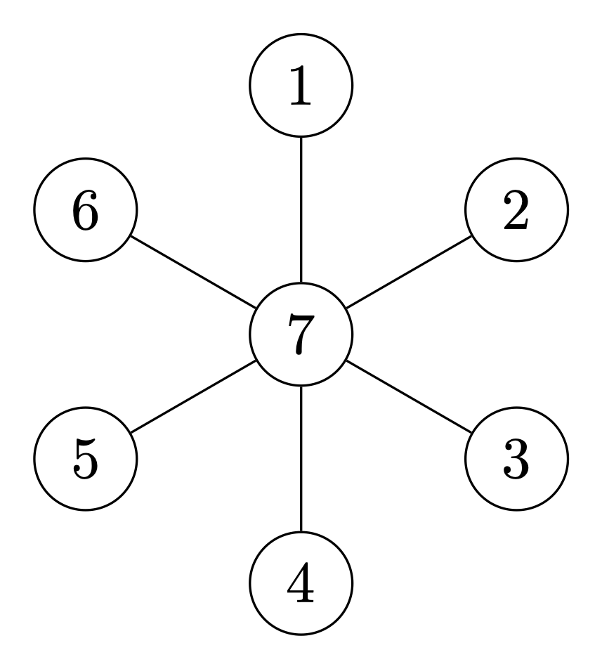
The introduced auxiliary variables (\(\alpha\)) can be viewed as simply adding additional nodes to the graph, and then letting the nodes "communicate" through these artificial nodes instead of to the other nodes directly. The reason why is possible is that a low-rank matrix represents that all flow in a graph is proportional.
In the case of \(A\) being diagonal and \(U\) and \(V\) being vectors, then the auxillary variable approach can be visualized as.
 In general one would need to add an extra node for each column in \(U\) (or \(V\)) and had \(A\) not been diagonal, then the edges stemming from its sparsity pattern would also be observed in the above graph.
Interpreting low-rank structure as prices
An analogical explanation of why low-rank additions has a structure that can be utilized for efficient computations is through prices of items in different currencies. Let \(x\) represent the number of items to buy, then the following analogous are true:
\(V\) are the prices of items (each column is a different currency).
\(U\) is the exchange rates of the prices given in \(V\) to other currencies.
\(UV^\top\) is prices of buying the items in the prices of \(V\) in the various currencies of \(U\).
\(U(V^\top x)\), states that we should first compute the total price of buying \(x\) items in the currencies of \(V\) (\(V^\top x\)) and then convert the total prices to the correct currencies described by exchange rates of \(U\). Notice that this is what anyone would do in practice.
The additional matrix \(A\) denotes some specific pricing differences between the countries for every item (taxations, import fees, shipping fees, etc.).