The Sherman-Morrison-Woodbury Identity

The Sherman-Morrison-Woodbury identity is the generalization of the Sherman-Morrison identity. In short, it says that the inverse of a rank-\(k\) perturbed matrix is also a rank-\(k\) perturbed matrix. Most notably it can be used to significantly speed up the computations of the inverse of the total matrix if the inverse of perturbed matrix is already known. This speedup is the main workhorse behind the efficiency of the BFGS algorithm (as it is based on a rank-2 update of the Hessian).

A Special Case

The derivation is simple. Assume the inverse have the form \(I + UZV^\top \), then we have that

\[\begin{aligned} (I + UV^\top )(I + UZV^\top ) & = I + (UV^\top + UZV^\top + UV^\top UZV^\top )\\ &= I + U(I + Z + V^\top UZ)V^\top . \end{aligned}\]

Since \(I + UZV^\top \) is assumed to be the inverse the above expression must be equal to \(I\). As a result we must have that

\[ I + Z + V^\top UZ = 0. \]

From this it follows that

\[ Z = (I + V^\top U)^{-1}(-I) = -(I + V^\top U)^{-1}. \]

As such we must have that \(Z\) is equal to the above in order for \(I + UZV^\top \) to be the actual inverse, which confirms the identity.

I sometimes find it easier to think of this identity in terms of visuals

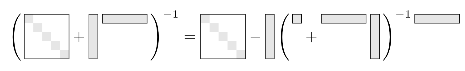
This clearly highlights how the identity can be used to reduce the problem of inverting a \(n\times n\) matrix to inverting a \(k\times k\) matrix at the expense of some matrix-vector products. If \(k \ll n\) then this reduction from \(O(n^3)\) to \(O(k^3 + kn)\) flops is a significant improvement.

The General Form

There exist several ways of showing this identity. The easiest is probably to set \(B = A + USV^\top \) so that \(B^{-1} = (I + A^{-1}USV^\top )^{-1}A^{-1}\). Now set \(W = A^{-1}U\) and \(Z^\top = SV^\top \) such that

\[ B^{-1} = \left(I + WZ^\top \right)^{-1}A^{-1}. \]

Now using the special case from the previous section we have that

\[\begin{aligned} B^{-1} &= \left(I - W(I+Z^\top W)^{-1}Z^\top \right)A^{-1}\\ &= \left(I - A^{-1}U(I+SV^\top A^{-1}U)^{-1}SV^\top \right)A^{-1}\\ &= A^{-1} - A^{-1}U(S^{-1}+V^\top A^{-1}U)^{-1}V^\top A^{-1}. \end{aligned}\]

An alternatively one can use a similar approach to the one presented in the previous section. The guess just has to be modified to the form \(A^{-1} + A^{-1}UZV^\top A^{-1}\). What is then left is to multiply with \((A + USV^\top )\), set the expression equal to \(I\) (because we assume that its an inverse) and isolate \(Z\).

Also in this case i like to think of the formula in terms of visuals

From this it is clear that we only get a speedup if the inverse of \(A^{-1}\) is already known. This might not seem useful, but it is actually the cornerstones of the Broyden–Fletcher–Goldfarb–Shanno algorithm. The speedup is in this case only from \(O(n^3)\) to \(O(k^3 + k(n^2 + n))\).

Code

The Julia library WoodburyMatrices.jl can be used to effeciently perform computations with Woodbury matrices.

using WoodburyMatrices, LinearAlgebra
n = 5000
k = 10
A = randn(n,n) + I
U = randn(n,k)
C = randn(k,k)
V = randn(n,k)
Woodbury_struct = Woodbury(A, U, C, V')
Woodbury_dense = A + U*C*V'
@time Woodbury_struct\ones(n)
@time Woodbury_dense\ones(n)

  3.100386 seconds (26 allocations: 572.549 MiB, 4.43% gc time)
  0.833070 seconds (8 allocations: 190.849 MiB, 0.99% gc time)

As expected we do not get a speed up as the inversion of the Sherman-Morrison-Woodbury matrix also requires us to invert a \(n\times n\) matrix. Thankfully the package supports a factorization of \(A\) instead of \(A\) directly. Using this a clear speed-up can be seen. Off course it is not a completely fair comparison as we have not included the time it takes to actually factorize \(A\).

n = 5000
k = 10
A = randn(n,n) + I
U = randn(n,k)
C = randn(k,k)
V = randn(n,k)
Woodbury_struct = Woodbury(lu(A), U, C, V')
Woodbury_dense = A + U*C*V'
@time Woodbury_struct\ones(n)
@time Woodbury_dense\ones(n)

  0.036912 seconds (14 allocations: 234.938 KiB)
  0.656523 seconds (8 allocations: 190.849 MiB, 0.60% gc time)

A Useful Consequence

This section is very noty and was mostly written because (8) was stated in some papers with only a reference to the Sherman-Morrison-Woodbury identity.

In the area of fast direct solvers a variation of the Sherman-Morrison-Woodbury formula is sometimes used. The motivation for this variant can be found in the fact that we need to invert \(S\) in the formula (5) which makes an immidiate hierarchical (recursive) computation of the inverse impossible. However the following variant takes care of this problem.

This variation can be derived by seeing that

\[ (S^{-1} + D^{-1})^{-1} = \left(D^{-1}(DS^{-1}D + D)D^{-1}\right)^{-1} = D(DS^{-1}D + D)^{-1}D. \]

Now applying the Sherman-Morrison-Woodbury formula to the inverse it follows that

\[\begin{aligned} \left(S^{-1} + D^{-1}\right)^{-1} &= D\left(D^{-1} - D^{-1}D\left(S + DD^{-1}D\right)^{-1}DD^{-1}\right)D\\ &= D\left(D^{-1} - \left(S + D\right)^{-1}\right)D.\\ \end{aligned}\]

Now inserting into (5) it follows that

\[\begin{aligned} (A + USV^\top )^{-1} &= A^{-1} - A^{-1}U(S^{-1} + D^{-1})^{-1}V^\top A^{-1}\\ &= A^{-1} - A^{-1}UD\left(D^{-1} - \left(S + D\right)^{-1}\right)DV^\top A^{-1}\\ &= \left(A^{-1} - A^{-1}UDV^\top A^{-1}\right) + A^{-1}UD\left(S + D\right)^{-1}DV^\top A^{-1} \end{aligned}\]

now setting \(E = A^{-1}UD\), \(F=(DV^\top A^{-1})^\top \) and \(G = A^{-1} - A^{-1}UDV^\top A^{-1}\) the variation of the Sherman-Morrison-Woodbury formula becomes apparent.