Cholesky factorization of an arrowhead matrix
The arrowhead example highlights why permutations are crucial when performing factorizations of sparse matrices. The example is from the book Convex Optimization by Stephen Boyd and Lieven Vandenberghe.
We start by defining two arrowhead matrices. One with the arrow pointing towards the top left (\(A_l\)) and one pointing towards the bottom right \((A_r)\)
\[ A_l = \begin{bmatrix} 1 & u^\top\\ u & \text{diag}(d) \end{bmatrix}, \quad A_r = \begin{bmatrix} \text{diag}(d) & u\\ u^\top & 1 \end{bmatrix}, \]where \(\text{diag}(d) \in \mathbb{R}^{n\times n}\) is a positive diagonal matrix and \(u \in \mathbb{R}^n\). In the case where \(u^\top\text{diag}(d)^{-1}u < 1\) the matrix is positive definite and a Cholesky factorization exist. For the left pointing arrowhead matrix the Cholesky factorization can be computed as
\[ A_l = \begin{bmatrix} 1 & u^\top\\ u & \text{diag}(d) \end{bmatrix} = \begin{bmatrix} 1 & 0\\ u & L \end{bmatrix} \begin{bmatrix} 1 & u^\top\\ 0 & L^\top \end{bmatrix}. \]Unfortunately looking at the bottom right block one find that \(LL^\top = \text{diag}(d) - uu^\top\). In general \(uu^\top\) will be dense meaning that \(L\) will also be a dense matrix. Visually we can represent the Cholesky factorization of the left pointing arrowhead matrix as 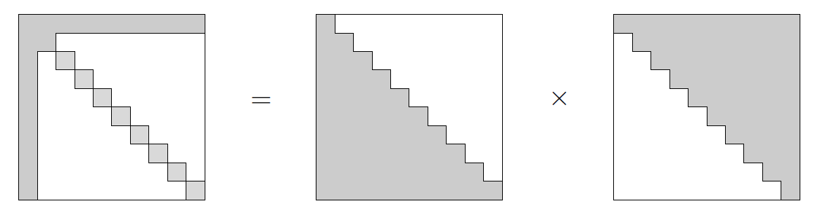
Surprisingly, the right pointing arrowhead matrix (which is simply a permutation of the left pointing arrowhead matrix) have a sparse Cholesky
\[ \begin{bmatrix} \text{diag}(d) & u\\ u^\top & 1 \end{bmatrix} = \begin{bmatrix} \text{diag}(d)^{1/2} & 0\\ u^\top \text{diag}(d)^{-1/2} & \sqrt{1 - u^\top \text{diag}(d)^{-1}u} \end{bmatrix} \begin{bmatrix} \text{diag}(d)^{1/2} & \text{diag}(d)^{-1/2}u\\ 0 & \sqrt{1 - u^\top \text{diag}(d)^{-1}u} \end{bmatrix}. \]Note that the above also shows why the constraint of \(u^\top\text{diag}(d)^{-1}u < 1\) was imposed earlier. We can similarly visualize the factorization as

Some Code
In most sparse linear algebra libraries the permutation of rows and columns happens automatically. To illustrate this a short example in Julia is given. We note here that the underlying sparse linear algebra library used in Julia is SuiteSparse (wrapped in SparseArrays.jl).
We start by setting up the problem as
using LinearAlgebra
using SparseArrays
n = 5
u = rand(n)
d = n./rand(n)
D = sparse(1:n,1:n,d)

Al = [1 u'; u D]
Ar = [D u; u' 1]

# Checking if Al and Ar are positive definite
u'*(D\u)
0.07854883491519178
Fl_dense = cholesky(Matrix(Al))6×6 LinearAlgebra.LowerTriangular{Float64, Matrix{Float64}}:
1.0 ⋅ ⋅ ⋅ ⋅ ⋅
0.331428 3.43691 ⋅ ⋅ ⋅ ⋅
0.602185 -0.0580699 9.45525 ⋅ ⋅ ⋅
0.0812995 -0.00783988 -0.00522595 2.97595 ⋅ ⋅
0.331309 -0.0319488 -0.0212966 -0.00917255 6.26863 ⋅
0.646985 -0.0623901 -0.0415883 -0.0179123 -0.0346799 2.52021Now computing the dense factorization of the right pointing arrowhead matrix (which is expected to be sparse)
Fr_dense = cholesky(Matrix(Ar))6×6 LinearAlgebra.LowerTriangular{Float64, Matrix{Float64}}:
3.45285 ⋅ ⋅ ⋅ ⋅ ⋅
0.0 9.47458 ⋅ ⋅ ⋅ ⋅
0.0 0.0 2.97707 ⋅ ⋅ ⋅
0.0 0.0 0.0 6.2775 ⋅ ⋅
0.0 0.0 0.0 0.0 2.6033 ⋅
0.0959868 0.063558 0.0273086 0.0527772 0.248525 0.959922In both case our expectations are verified.
We now redo the computations using a sparse factorization
Fl = cholesky(Al)6×6 SparseArrays.SparseMatrixCSC{Float64, Int64} with 11 stored entries:
2.6033 ⋅ ⋅ ⋅ ⋅ ⋅
⋅ 6.2775 ⋅ ⋅ ⋅ ⋅
⋅ ⋅ 2.97707 ⋅ ⋅ ⋅
⋅ ⋅ ⋅ 9.47458 ⋅ ⋅
⋅ ⋅ ⋅ ⋅ 3.45285 ⋅
0.248525 0.0527772 0.0273086 0.063558 0.0959868 0.959922Fr = cholesky(Ar)6×6 SparseArrays.SparseMatrixCSC{Float64, Int64} with 11 stored entries:
2.6033 ⋅ ⋅ ⋅ ⋅ ⋅
⋅ 6.2775 ⋅ ⋅ ⋅ ⋅
⋅ ⋅ 2.97707 ⋅ ⋅ ⋅
⋅ ⋅ ⋅ 9.47458 ⋅ ⋅
⋅ ⋅ ⋅ ⋅ 3.45285 ⋅
0.248525 0.0527772 0.0273086 0.063558 0.0959868 0.959922Notably the sparse factorization is in both cases found. The reason here being the permutations (which can be extracted from the factorizations using .p)
show(stdout, "text/plain", Fl.p)
show(stdout, "text/plain", Fr.p)
6-element Vector{Int64}:
6
5
4
3
2
1
6-element Vector{Int64}:
5
4
3
2
1
6Notice that the permutation heuristic in this case also end up reversing the entries of the diagonal matrix. However, the same final permutation is found for both the left and right pointing arrowhead matrices.
show(stdout, "text/plain", Al[Fl.p,Fl.p])6×6 SparseArrays.SparseMatrixCSC{Float64, Int64} with 16 stored entries:
6.77718 ⋅ ⋅ ⋅ ⋅ 0.646985
⋅ 39.407 ⋅ ⋅ ⋅ 0.331309
⋅ ⋅ 8.86296 ⋅ ⋅ 0.0812995
⋅ ⋅ ⋅ 89.7677 ⋅ 0.602185
⋅ ⋅ ⋅ ⋅ 11.9222 0.331428
0.646985 0.331309 0.0812995 0.602185 0.331428 1.0show(stdout, "text/plain", Ar[Fr.p,Fr.p])6×6 SparseArrays.SparseMatrixCSC{Float64, Int64} with 16 stored entries:
6.77718 ⋅ ⋅ ⋅ ⋅ 0.646985
⋅ 39.407 ⋅ ⋅ ⋅ 0.331309
⋅ ⋅ 8.86296 ⋅ ⋅ 0.0812995
⋅ ⋅ ⋅ 89.7677 ⋅ 0.602185
⋅ ⋅ ⋅ ⋅ 11.9222 0.331428
0.646985 0.331309 0.0812995 0.602185 0.331428 1.0