The Method of Moving Asymptotes
The Method of Moving Asympotes (MMA) can be used to solve inequality constrained optimization problems like the one below
\[\begin{aligned} \min_{\mathbf{x} \in\mathbb{R}^n} \quad f_0(\mathbf{x})&\\ f_i(\mathbf{x}) \leq \hat{f}_i, \quad &\text{for } i=1,\dots, m\\ x_j^{l} \leq x_j \leq x_j^u, \quad &\text{for } j=1,\dots, n. \end{aligned}\]The main idea behind the algorithm is to substitute all functions \(f_i\) by first order convex approximations. More specifically we approximate the functions using translations of the multiplicative inverse function. This can be done as follows:
Given a iteration point \(\mathbf{x}^{(k)}\), choose parameters \(L_j^{(k)}\) and \(U_j^{(k)}\) satisfying
\[ L_j^{(k)} < x_j^{(k)} < U_j^{(k)}, \quad j = 1,\dots n, \]then calculate the convex approximation of all functions \(f_i(\mathbf{x})\) as
\[ f_i^{(k)}(\mathbf{x}) = r_i^{(k)} + \sum_{j=1}^n \left(\frac{p_{ij}^{(k)}}{U_j^{(k)}-x_j} + \frac{q_{ij}^{(k)}}{x_j-L_j^{(k)}} \right). \]Where
\[\begin{aligned} p_{ij}^{(k)} &= \begin{cases} (U_j^{(k)}-x_j^{(k)})^2\frac{\partial f_i}{\partial x_j}, \qquad \hspace{-3pt} &\text{if }\frac{\partial f_i}{\partial x_j} > 0\\ 0, & \text{if } \frac{\partial f_i}{\partial x_j} \leq 0 \end{cases},\\ q_{ij}^{(k)} &= \begin{cases} 0, & \text{if }\frac{\partial f_i}{\partial x_j} \geq 0\\ -(x_j^{(k)}-L_j^{(k)})^2\frac{\partial f_i}{\partial x_j}, \quad &\text{if } \frac{\partial f_i}{\partial x_j} < 0 \end{cases},\\ r_i^{(k)} &= f_i(\mathbf{x}^{(k)}) - \sum_{j=1}^n \left(\frac{p_{ij}^{(k)}}{U_j^{(k)}-x_j} + \frac{q_{ij}^{(k)}}{x_j-L_j^{(k)}} \right). \end{aligned}\]Note that all derivatives \(\frac{\partial f_i}{\partial x_j}\) are evaluated at \(\mathbf{x} = \mathbf{x}^{(k)}\). By the above definitions of \(p_{ij}^{(k)}\) and \(q_{ij}^{(k)}\), we see that the sum in (3) for each \(j\) only contain either the term with \(p_{ij}^{(k)}\) or the term with \(q_{ij}^{(k)},\) hence we only have one asymptote for each \(f_i\). Furthermore it is easy to see that \(f_i^{(k)}(\mathbf{x})\) is a first order approximation of \(f_i(\mathbf{x})\) at \(\mathbf{x}^{(k)}\), i.e that it is satisfied that
\[ f_i^{(k)}(\mathbf{x}^{(k)}) = f_i(\mathbf{x}^{(k)}) \quad \text{and} \quad \frac{\partial f_i^{(k)}}{\partial x_j} = \frac{\partial f_i}{\partial x_j} \text{ at }\mathbf{x} = \mathbf{x}^{(k)}, \]for \(i=0,1,\dots, m\) and \(j=1,\dots, n\).
The final convex subproblem \(P^{(k)}\) can now be stated simply as
\[\begin{aligned} \min_{\mathbf{x} \in\mathbb{R}^n} \quad &r_0^{(k)} + \sum_{j=1}^n \left(\frac{p_{0j}^{(k)}}{U_j^{(k)}-x_j} + \frac{q_{0j}^{(k)}}{x_j-L_j^{(k)}} \right), \\ &r_i^{(k)} + \sum_{j=1}^n \left(\frac{p_{ij}^{(k)}}{U_j^{(k)}-x_j} + \frac{q_{ij}^{(k)}}{x_j-L_j^{(k)}} \right) \leq \hat{f}_i, \quad\ \text{for } i=1,\dots, m\\ &\max\{x_j^{l},\alpha_j^{(k)}\} \leq x_j \leq \min\{x_j^u, \beta_j^{(k)}\}, \quad\ \quad\ \quad \text{for } j=1,\dots, n. \end{aligned}\]Here the variables \(\alpha_j^{(k)}\) and \(\beta_j^{(k)}\) is introduced to make sure that no divisibility by zero occur, hence they should be chosen such that
\[ L_j^{(k)} < \alpha_j^{(k)} < x_j^{(k)} < \beta_j^{(k)} < U^{(k)}_j. \]In [1] it is proposed to set \(\alpha_j^{(k)} = 0.9L_j^{(k)} + 0.1x_j^{(k)}\) and \(\beta_j^{(k)} = 0.9U_j^{(k)}+0.1x_j^{(k)}\).
A important part of the algorithm is however yet to be described, namely the part of moving the asymptotes. The idea is as follows. a) If the algorithm oscillates, then it can be stabilized by moving the asymptotes closer to the iteration point. b) If the algorithm is monotone, then it can be relaxed by moving the asymptotes further from the iteration point.
There exist many implementations of the above but a proposed implementation from ?? is to chose \(s\in ]0,1[\) and then do the following.
For \(k \leq 1\) let
For \(k \geq 2\) then a) If the signs of \(x_j^{(k)}-x_j^{(k-1)}\) and \(x_j^{(k)}-x_j^{(k-1)}\) differ then let
\[ L_j^{(k)} = x_j^{(k)} - s(x^u_j - x^l_j)\ \text{ and }\ U_j^{(k)} = x_j^{(k)} + s(x^u_j - x^l_j). \]b) If the signs of \(x_j^{(k)}-x_j^{(k-1)}\) and \(x_j^{(k)}-x_j^{(k-1)}\) are the same then let
\[ L_j^{(k)} = x_j^{(k)} - (x^u_j - x^l_j)/s\ \text{ and }\ U_j^{(k)} = x_j^{(k)} + (x^u_j - x^l_j)/s. \]Cones
Transforming the convex subproblem into a conic form, such that the convexity is given directly from the problem formulation. In order to do so the rotated quadratic cone in three dimension is used.
\[ \mathcal{Q}_r^3 = \{ \mathbf{x}\in\mathbb{R}^3\ |\ 2x_1x_2 \geq x_3^2\}. \]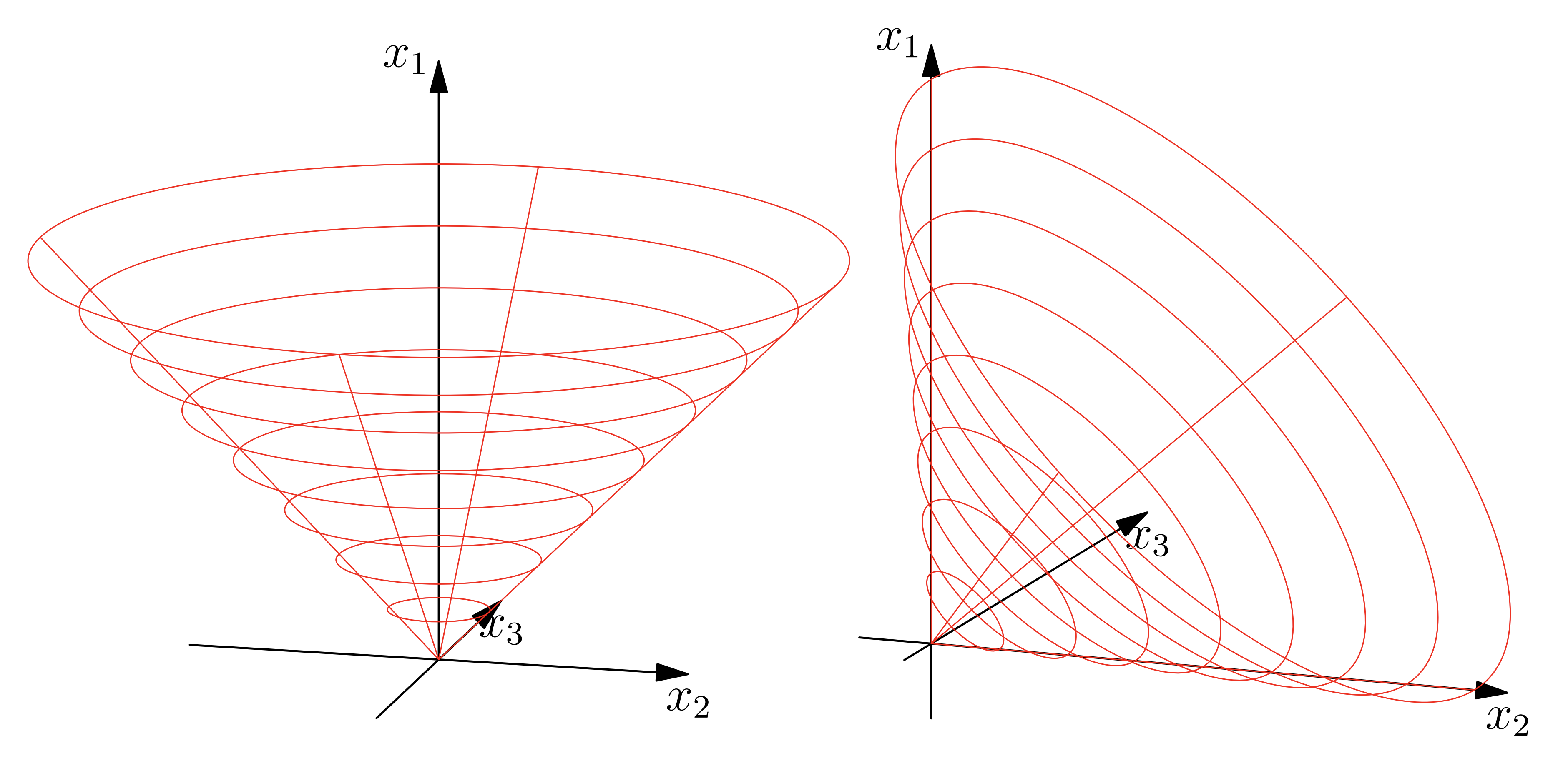
The idea is to introduce a rotated quadratic cone for each asymptote in the convex approximations as each asymptote will have the following epigraph form.
\[ s_{ij}\frac{p_{ij}}{U_j-x_j} + (1-s_{ij})\frac{q_{ij}}{x_j - L_j} \leq t_{ij}, \]where \(t_{ij}\) is an auxiliary variable and \(s_{ij}\) is a binary value describing if the upper or lower asymptotes is active or not. Abusing this notation we can rewrite the inequality as
\[ s_{ij}p_{ij} + (1-s_{ij})q_{ij} \leq t_{ij}\left(s_{ij}(U_j-x_j) + (1-s_{ij})(x_j - L_j) \right). \]Now using the definition of the rotated quadratic cone as described in (11) get that
\[ \begin{bmatrix} %\frac{t_{ij}}{2}\\ t_{ij}\\ s_{ij}(U_j-x_j) + (1-s_{ij})(x_j - L_j)\\ \sqrt{2}\sqrt{p_{ij}s_{ij} + (1-s_{ij})q_{ij}} \end{bmatrix} \in \mathcal{Q}_r^3, \quad \text{for } i = 0,1,\dots m,\text{ and } j=1,\dots, n. \]The final optimization problem is given below.
\[\begin{aligned} \min_{x\in\mathbb{R}^n, t\in \mathbb{R}^{m\cdot n}, z\in\mathbb{R}} z \qquad&\\ 0 \leq t_{ij} \qquad \text{for } &i = 0,1,\dots m,\text{ and } j=1,\dots, n.\\ \sum_{j=1}^m t_{ij} \leq z, \quad \text{ for } &i=0,1,\dots, n.\\ \begin{bmatrix} %\frac{t_{ij}}{2}\\ t_{ij}\\ s_{ij}(U_j-x_j) + (1-s_{ij})(x_j - L_j)\\ \sqrt{2}\sqrt{p_{ij}s_{ij} + (1-s_{ij})q_{ij}} \end{bmatrix} \in \mathcal{Q}_r^3, \quad \text{for } &i = 0,1,\dots m,\text{ and } j=1,\dots, n.\\ x_j^{l} \leq x_j \leq x_j^u, \quad \text{for } &j=1,\dots, n. \end{aligned}\]The above optimization problem can be solved using a conic solver such as MOSEK.
References
| [1] | Svanberg, Krister. “The method of moving asymptotes - A new method for structural optimization.” International Journal for Numerical Methods in Engineering 24.2 (1987): 359–373. Print. |