The Fast Multipole Method for Boundary Elements

I often find that texts regarding the Boundary Element Method mentions how the Fast Multipole Method can be utilized to get rid of the \(\mathcal{O}(n^2)\) memory and computational scalings of the BEM. While there exist many good introductory text to the Fast Multipole Method (FMM) such as for example Lexing Yings A pedstrian introduction to fast multipole methods ^[1], no such text can be found for their application to the BEM. As such this note serves as a brief description of how to apply the FMM to speed up BEM computations.

The specifics of the implementation will depend on the underlying FMM library used. In this note I will stick to the approach taken in the Flatiron Institute Fast Multipole Libraries^[2], where the representational formula has the following form

\[ u(\mathbf{x}) = \sum_{j=1}^M\left[c_j\frac{\mathrm{e}^{\mathrm{i} k\|\mathbf{x} - \mathbf{x}_j\|}}{\|\mathbf{x} - \mathbf{x}_j\|} - \mathbf{v}_j\cdot\nabla\left(\frac{\mathrm{e}^{\mathrm{i} k\|\mathbf{x} - \mathbf{x}_j\|}}{\|\mathbf{x} - \mathbf{x}_j\|}\right)\right], \]

where when \(\mathbf{x} = \mathbf{x}_j\) the \(j\)th term is excluded from the sum. Note that in both terms are missing the standard \((4\pi)^{-1}\), meaning that from an implementation point of view this constant needs to be added to the values of \(c_j\) and \(\mathbf{v}_j\).

Implementation overview

Depending on the chosen Boundary Element scheme the specifics of how to apply the Fast Multipole Method to speed up the computations changes. However, they are all based on the same principles of splitting the BE matrix, \(\mathbf{A}\), into parts which are either sparse or can be approximated using the FMM. For the three main types of BE discretizations the splitting looks as follows

1. Nyström

\[ \mathbf{A} = \mathbf{G} - \mathbf{C} + \mathbf{S}, \quad \mathbf{A}\in\mathbb{C}^{N\times N} \]

2. Collocation

\[ \mathbf{A} = (\mathbf{G} -\mathbf{C})\mathbf{F} +\mathbf{S} = \mathbf{G}\mathbf{F} - \widetilde{\mathbf{C}} + \mathbf{S}, \quad \mathbf{G}, \mathbf{C}\in\mathbb{C}^{N\times M},\ \mathbf{F}\in\mathbb{C}^{M\times N}, \mathbf{S}\in\mathbb{C}^{N\times N} \]

3. Galerkin

\[ \mathbf{A} = \mathbf{F}^\top(\mathbf{G} - \mathbf{C})\mathbf{F} + \mathbf{S} = \mathbf{F}^\top \mathbf{G} \mathbf{F} - \widetilde{\mathbf{C}} + \mathbf{S}, \quad \mathbf{G}, \mathbf{C}\in\mathbb{C}^{M\times M},\ \mathbf{F}\in\mathbb{C}^{M\times N}, \mathbf{S}\in\mathbb{C}^{N\times N} \]

In the above the matrix \(\mathbf{G}\) is the one approximated using e.g. FMM or an \(\mathcal{H}\)-matrix, we then subtract \(\mathbf{C}\) which represents the numerical inaccuracies from close-to-singular points included in \(\mathbf{G}\) while \(\mathbf{S}\) corresponds to the correct singular integration of the same close-singular-points. This means that the combination \(-\widetilde{\mathbf{C}} + \mathbf{S}\) can be viewed as representing the correction of the nearfield interactions. Lastly the matrix \(\mathbf{F}\) acts as a map from the nodal values to the gaussian points used in the approximation schemes. In all cases \(\mathbf{C}, \mathbf{S}\) and \(\mathbf{F}\) are highly sparse matrices, meaning that both assembly and multiplication with these should scale \(\mathcal{O}(n\tau)\) where \(\tau \ll n\). This means that using an approximate scheme for \(\mathbf{G}\) with a multiplication that scales linear in time and memory we have a representation of \(\mathbf{A}\) that also scale linear in time and memory.

Handling Singular Integration

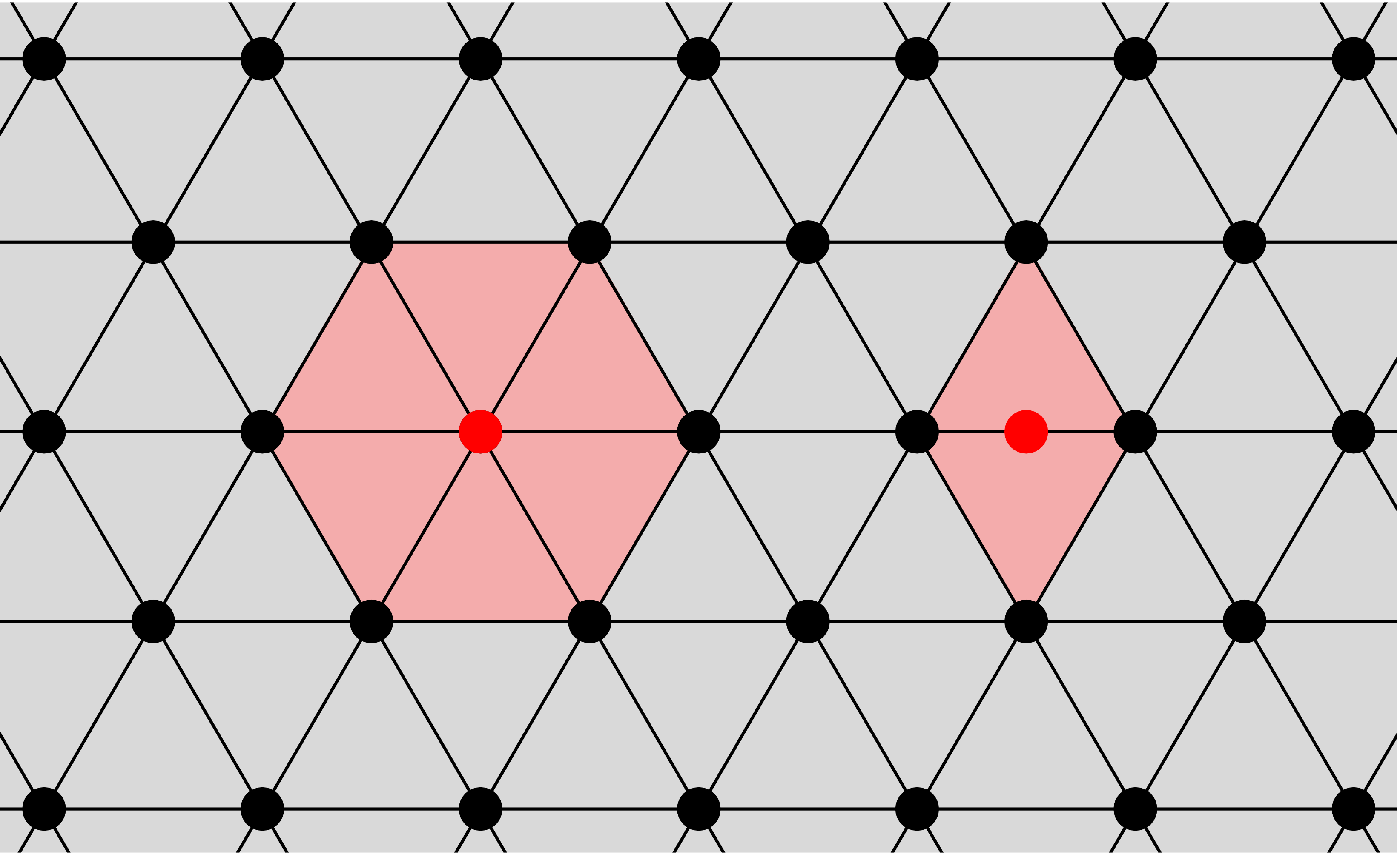
As mentioned previously \(-\widetilde{\mathbf{C}} + \mathbf{S}\) serves as a correction of the nearfield computations. In the case of collocation this correction step requires the recomputation of the part of the integrals that corresponds to the surrounding elements. For a corner and edge node these elements can be seen below (where the red dots represents the corner and edge node respetively).

How to use the representation formula

When solving BEM we are interested in integrals of the form

\[ \int_\Gamma G(\mathbf{x},\mathbf{y})\mathbf{N}(\mathbf{x})^\top \frac{\partial \mathbf{p}}{\partial\mathbf{n} }\ \mathrm{d}\Gamma_\mathbf{x} = \sum_{j=1}^{N_{elements}}\int_{\Gamma_j} G(\mathbf{x},\mathbf{y})\mathbf{N}(\mathbf{x})^\top \frac{\partial \mathbf{p}}{\partial\mathbf{n} }\ \mathrm{d}\Gamma_\mathbf{x}, \] \[ \int_\Gamma \mathbf{n} \cdot \left[\nabla G(\mathbf{x},\mathbf{y})\right]\mathbf{N}(\mathbf{x})^\top \mathbf{p}\ \mathrm{d}\Gamma_\mathbf{x} = \sum_{j=1}^{N_{elements}}\int_{\Gamma_j} \mathbf{n} \cdot \left[\nabla G(\mathbf{x},\mathbf{y})\right]\mathbf{N}(\mathbf{x})^\top \mathbf{p}\ \mathrm{d}\Gamma_\mathbf{x}. \]

The standard way of approximating these integrals is using so-called gaussian quadrature, meaning that the above can be further written as

\[ \sum_{j=1}^{N_{elements}}\int_{\Gamma_j} G(\mathbf{x},\mathbf{y})\mathbf{N}(\mathbf{x})^\top \frac{\partial \mathbf{p}}{\partial\mathbf{n} }\ \mathrm{d}\Gamma_\mathbf{x} \approx \sum_{j=1}^{N_{elements}}\sum_{\ell=1}^{n_{gauss}} G(\mathbf{x}_\ell,\mathbf{y})\mathbf{N}(\mathbf{x}_\ell)^\top \frac{\partial \mathbf{p}}{\partial\mathbf{n} }, \] \[ \sum_{j=1}^{N_{elements}}\int_{\Gamma_j} \mathbf{n} \cdot \left[\nabla G(\mathbf{x},\mathbf{y})\right]\mathbf{N}(\mathbf{x})^\top \mathbf{p}\ \mathrm{d}\Gamma_\mathbf{x} \approx \sum_{j=1}^{N_{elements}}\sum_{\ell=1}^{n_{gauss}} \mathbf{n}_\ell \cdot \left[\nabla G(\mathbf{x}_\ell,\mathbf{y})\right]\mathbf{N}(\mathbf{x}_\ell)^\top \mathbf{p}\ \mathrm{d}\Gamma_\mathbf{x} \]

References

[1]	Ying, L. (2012). A pedestrian introduction to fast multipole methods. doi: 10.1007/s11425-012-4392-0

[2]	Flatiron Institute Fast Multipole Libraries.