Boundary Layer Impedance

The inclusion of viscothermal losses in acoustical computations can be approximated using the so-called Boundary Layer Impedance (BLI) approach described by ^[1]. Here the viscothermal effects are approximated by applying a Wentzell (Venttsel') type boundary condition. Using the description from ^[2] the boundary condition have the following form

\[ \frac{\partial p}{\partial \mathbf{n}} = \left[(\gamma - 1)\frac{\mathrm{i} k^2}{k_h} -\frac{\mathrm{i}\Delta_{\text{T}}}{k_v}\right]p, \]

where \(\gamma\) is the heat capacity ratio and \(k, k_v, k_h\) are the respectively the standard, viscous and thermal wavenumbers. Splitting up the double-layer potential into a part with a standard velocity condition (\(\Gamma_\text{io}\) in the figure) and a part with a BLI condition (\(\Gamma_\text{BLI}\) in the figure) we find that

\[ \begin{aligned} c(\mathbf{x})p(\mathbf{x}) = \int_{\Gamma_{\text{io}}} G(\mathbf{x},\mathbf{y})\frac{\partial p(\mathbf{y})}{\partial \mathbf{n}_\mathbf{y}}\ \mathrm{d}S_\mathbf{y} - \int_\Gamma\frac{\partial G(\mathbf{x},\mathbf{y})}{\partial \mathbf{n}_\mathbf{y}}&p(\mathbf{y})\ \mathrm{d}S_\mathbf{y} \\ +\int_{\Gamma_{\text{BLI}}} G(\mathbf{x},\mathbf{y})\left[ \frac{(\gamma - 1)\mathrm{i} k^2}{k_h} -\frac{\mathrm{i}\Delta_{\text{T}} }{k_v}\right]&p(\mathbf{y})\ \mathrm{d}S_\mathbf{y}. \end{aligned} % c(\mathbf{x})p(\mathbf{x}) = \int_{\Gamma_{\text{io}}} G(\mathbf{x},\mathbf{y})\frac{\partial p(\mathbf{y})}{\partial \mathbf{n}_\mathbf{y}}\ \mathrm{d}S_\mathbf{y} - \int_\Gamma\frac{\partial G(\mathbf{x},\mathbf{y})}{\partial \mathbf{n}_\mathbf{y}}p(\mathbf{y})\ \mathrm{d}S_\mathbf{y} % +\int_{\Gamma_{\text{BLI}}} G(\mathbf{x},\mathbf{y})\left[ \frac{(\gamma - 1)\mathrm{i} k^2}{k_h} -\frac{\mathrm{i}\Delta_{\text{T}} }{k_v}\right]p(\mathbf{y})\ \mathrm{d}S_\mathbf{y}. \]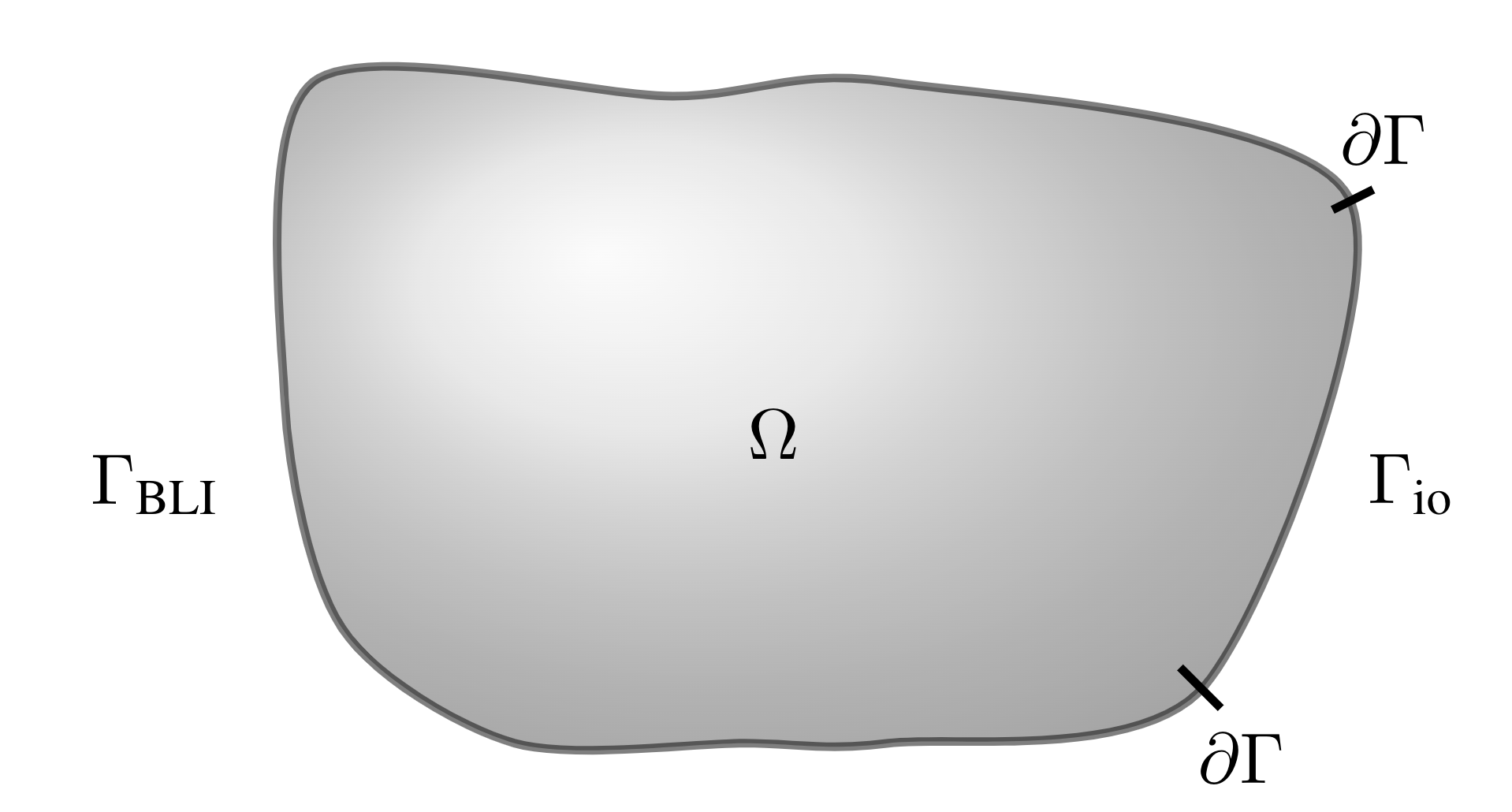

Applying integration by parts to the term including \(\Delta_\text{T}\) in (2) while assuming that

\[ \int_{\partial\Gamma_{\text{BLI}}} G(\mathbf{x},\mathbf{y})\frac{\partial p(\mathbf{y})}{\partial\mathbf{n}_\mathbf{y}}\ \mathrm{d}S_\mathbf{y} = 0, \]

it follows that

\[ \begin{aligned} c(\mathbf{x})p(\mathbf{x}) = \int_{\Gamma_{\text{io}}} G(\mathbf{x},\mathbf{y})\frac{\partial p(\mathbf{y})}{\partial \mathbf{n}_\mathbf{y}}\ \mathrm{d}S_\mathbf{y} - \int_\Gamma\frac{\partial G(\mathbf{x},\mathbf{y})}{\partial \mathbf{n}_\mathbf{y}}&p(\mathbf{y})\ \mathrm{d}S_\mathbf{y}\\ + \frac{(\gamma - 1)\mathrm{i} k^2}{k_h}\int_{\Gamma_{\text{BLI}}}G(\mathbf{x},\mathbf{y})&p(\mathbf{y})\ \mathrm{d}S_\mathbf{y} + \frac{\mathrm{i}}{k_v}\int_{\Gamma_{\text{BLI}}} \nabla_{\text{T}} G(\mathbf{x},\mathbf{y})\cdot \nabla_{\text{T}} p(\mathbf{y})\ \mathrm{d}S_\mathbf{y}. \end{aligned} \]

Note that the assumption of (3) is described in detail in section 4 of ^[1]. According to the definition of the tangential (surface) gradient it further reduces that

\[ \nabla_{\text{T}}G\cdot\nabla_{\text{T}}p = \left(\nabla G - \frac{\partial G}{\partial \mathbf{n}}\mathbf{n}\right)^\top\left(\nabla p - \frac{\partial p}{\partial \mathbf{n}}\mathbf{n}\right) %=\nabla_xG\cdot\nabla_xp - \frac{\partial G}{\partial \mathbf{n}}\frac{\partial p}{\partial \mathbf{n}} = \left(\nabla G - \frac{\partial G}{\partial\mathbf{n}}\mathbf{n}\right)^\top\nabla p. \]

Consequently inserting the above into (4) we attain the final form of the underlying model of interest in this paper

\[ \begin{aligned} c(\mathbf{x})p(\mathbf{x}) &= \int_{\Gamma_{\text{io}}} G(\mathbf{x},\mathbf{y})\frac{\partial p(\mathbf{y})}{\partial \mathbf{n}_\mathbf{y}}\ \mathrm{d}S_\mathbf{y} - \int_\Gamma\frac{\partial G(\mathbf{x},\mathbf{y})}{\partial \mathbf{n}_\mathbf{y}}p(\mathbf{y})\ \mathrm{d}S_\mathbf{y}\\ &+\frac{(\gamma - 1)\mathrm{i} k^2}{k_h}\int_{\Gamma_{\text{BLI}}}G(\mathbf{x},\mathbf{y})p(\mathbf{y})\ \mathrm{d}S_\mathbf{y} + \frac{\mathrm{i}}{k_v}\int_{\Gamma_{\text{BLI}}} \left(\nabla_\mathbf{y} G(\mathbf{x},\mathbf{y}) - \frac{\partial G}{\partial\mathbf{n}_\mathbf{y}}\mathbf{n_\mathbf{y}}\right)^\top\nabla p(\mathbf{y})\ \mathrm{d}S_\mathbf{y}. \end{aligned} \]

Following the discretization procedure described in the previous section one finds that the above can be represented as the following linear system of equations

\[ \text{diag}(\mathbf{c})\mathbf{p} = \mathbf{G}_{\Gamma_{\text{io}}}\frac{\partial\mathbf{p}}{\partial \mathbf{n}} - \mathbf{F}\mathbf{p} + \frac{(\gamma - 1)\mathrm{i} k^2}{k_h}\mathbf{H}_{\Gamma_{\text{BLI}}}\mathbf{p} + \frac{\mathrm{i}}{k_v}\mathbf{T}_{\Gamma_\text{BLI}}\mathbf{p}. \]

Again applying boundary conditions will result in a linear system of equations

\[ \mathbf{A}\mathbf{z} = \mathbf{b}, \]

where \(\mathbf{z}\) is a vector containing nodal values of either \(p\) or \(\partial_\mathbf{n} p\).

References

[1]	Berggren, Martin, et al. “Acoustic Boundary Layers as Boundary Conditions.” Journal of Computational Physics, vol. 371, Academic Press Inc., 2018, pp. 633–50, doi:10.1016/j.jcp.2018.06.005.

[2]	Risby Andersen, Peter, Cutanda Henriquez, Vicente & Aage, Niels. "On the validity of numerical models for viscothermal losses in structural optimization for micro-acoustics", PrePrint