Line Elements
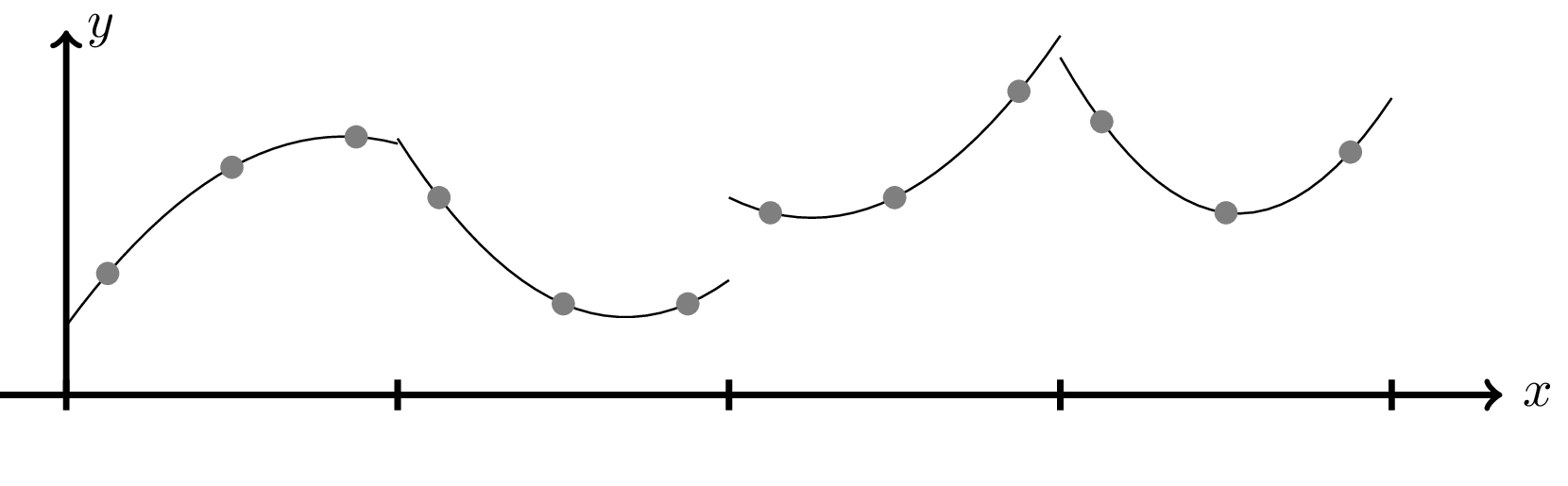
In this not we look into so-called line elements which are used for the one-dimensional Finite Element Method (FEM) and two-dimensional Boundary Element Method (BEM). In both cases there are two discretizations happening:
Discretization of the geoemetry
The reason for this is simply that parametrization of curves in general can be difficult. The job of this discretization is to split the curve of interest into smaller subcurves (elements) which can be described using simple functions such as polynomials. In fact in this small node we only focus on polynomial elements. This is mostly a problem for the BEM
Discretization of the physics
The reason for this is that we aim to parametrize a family of functions for which we hope to find a solution to our PDE. This can be done in various ways but in this note we only look at polynomial parametrization. Firstly we look at so-called continuous schemes of which the physics follows the geometric nodes and discontinuous schemes where the physics follow the elements.
In practice the discretization of the geometry is done by introducing a matrix \(\mathbf{X}\) which has columns equal to the points that we want the curve to connect (note that some implementations have the points as rows)
\[ \mathbf{X} = \begin{bmatrix} \mathbf{x}_1 & \mathbf{x}_2 & \dots & \mathbf{x}_n \end{bmatrix}. \]The idea is that we can now parametrize the curve of interest as
\[ \mathbf{x}(u) = \mathbf{X}\mathbf{T}_\mathbf{x}(u), \]where \(\mathbf{T}_\mathbf{x}(u)\) is a vector function which represents the interpolation between each geometric node \(\mathbf{x}_i\). In practice, however, it is usually more easy to introduce the so-called topology matrix (also sometimes called a connectivity matrix) as
\[ \left. \text{topology} = \begin{bmatrix} 1 & 2 & \dots & n-2 & n-1 \\ 2 & 3 & \dots & n-1 & n \end{bmatrix} \right\}\text{Connectivity matrix of coordinates}, \]where each column represents an element. What this means is that the values in a column represents node-numbers which is interpolated between on said element.
The discetization of the physics is similar, namely that we introduce the following vector \(\mathbf{p}\) which contains the nodal values \(p_i\) as
\[ \mathbf{p} = \begin{bmatrix} p_1 \\ p_2 \\ \vdots \\ p_n. \end{bmatrix} \]Using these nodal values we can create an interpolation of them in the same way as for the geometrical nodes
\[ p(x) = \mathbf{T}_p(x)\mathbf{p}. \]Note that in many cases it has been chosen to set \(\mathbf{T}_\mathbf{x} = \mathbf{T}_p\) since it simplifies the implementation. A key insight into element methods is that (5) serves a parametrization of possible solutions to the PDE of interest. Both FEM and BEM are then based on setting up a linear system of equation in order to find \(\mathbf{p}\) such that (5) is the best possible approximation of solution with respect to some chosen error measure.
Continuous
In the following we only visualize 1-dimensional problems, but its important to note that everything discussed is directly translatable into n-dimensional curves. The only difference here being that the number of rows in \(\mathbf{X}\) is equal to the dimension of interest.
Linear
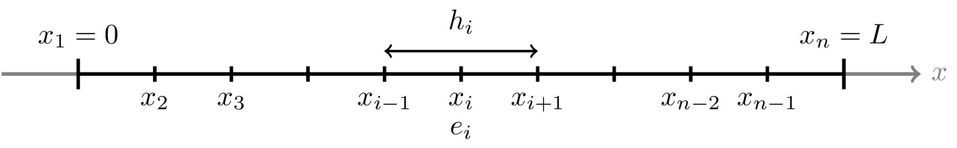
We start by dividing the domain \(\Omega = [0,L]\) into elements as 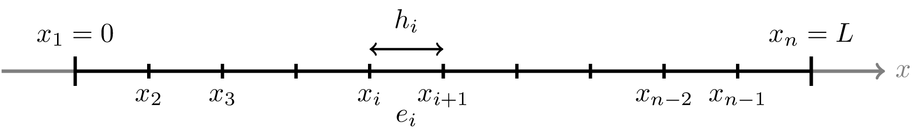
Here \(x_i\) are called nodes (also called points), \(e_i\) represents element \(i\) and \(h_i = x_{i+1} - x_i\) is the element length. The connectivity of these elements can be described by the following topology matrix
\[ \text{topology} = \begin{bmatrix} 1 & 2 & \dots & n-2 & n-1 \\ 2 & 3 & \dots & n-1 & n \end{bmatrix} \]Now we want to find the basis functions (also denoted interpolation functions or shape functions) on element \(i\) such that the interpolation between \(x_i\) and \(x_{i+1}\) is linear. Firstly the lineariry mean that
\[ T_i(x)x_i + T_{i+1}(x)x_{i+1} = ax + b, \quad x\in [x_i, x_{i+1}]. \]Now since we want this to interpolate between \(x_i\) and \(x_{i+1}\) we must have that
\[ \begin{aligned} T_i(x_i)x_i + T_{i+1}(x_i)x_{i+1} = ax_i + b &= x_i,\\ T_i(x_{i+1})x_i + T_{i+1}(x_{i+1})x_{i+1} = ax_{i+1}+ b &= x_{i+1}. \end{aligned} \]Since we have two equation and two unkowns (\(a,b\)) we can solve for the unkowns and rearrange such that
\[ \begin{aligned} T_i(x)x_i + T_{i+1}(x)x_{i+1} = x_i\left(\frac{x_{i+1}-x}{h_i}\right) + x_{i+1}\left(\frac{x-x_i}{h_i}\right). \end{aligned} \]Now a crucial comment is that the above is only true when have \(x\in[x_i,x_{i+1}]\) (i.e. when \(x\) is on element \(i\)) it is there custom to instead write
\[ T_i^1(x)x_i + T_i^2(x)x_{i+1}, \]where \(T_i^1(x)=T_i^2(x) = 0\) when \(x\notin [x_i, x_{i+1}]\). 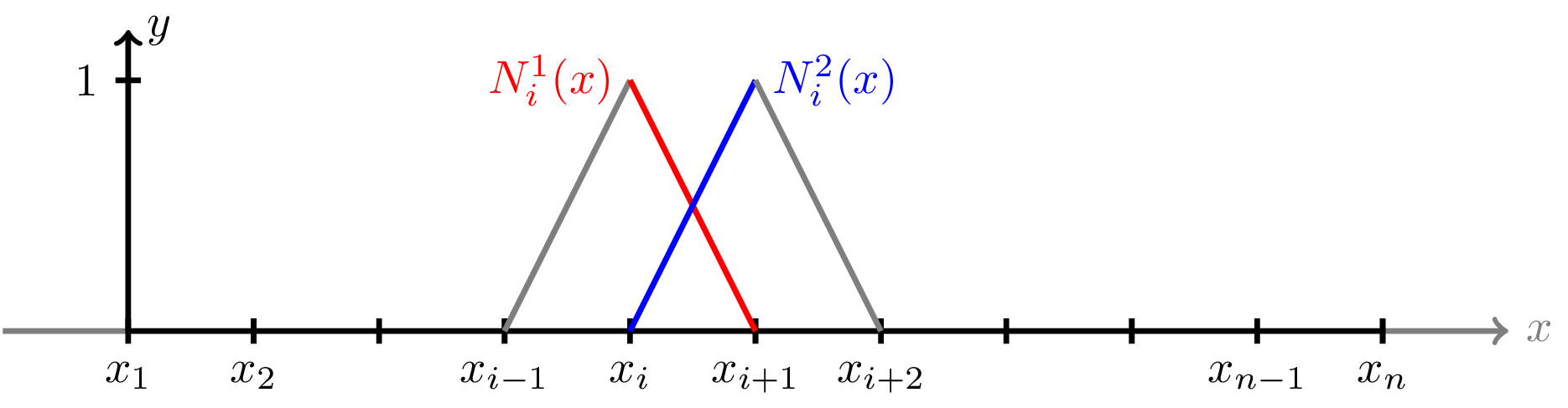
Now given the topology of the elements it is easy to extend the above results to the following 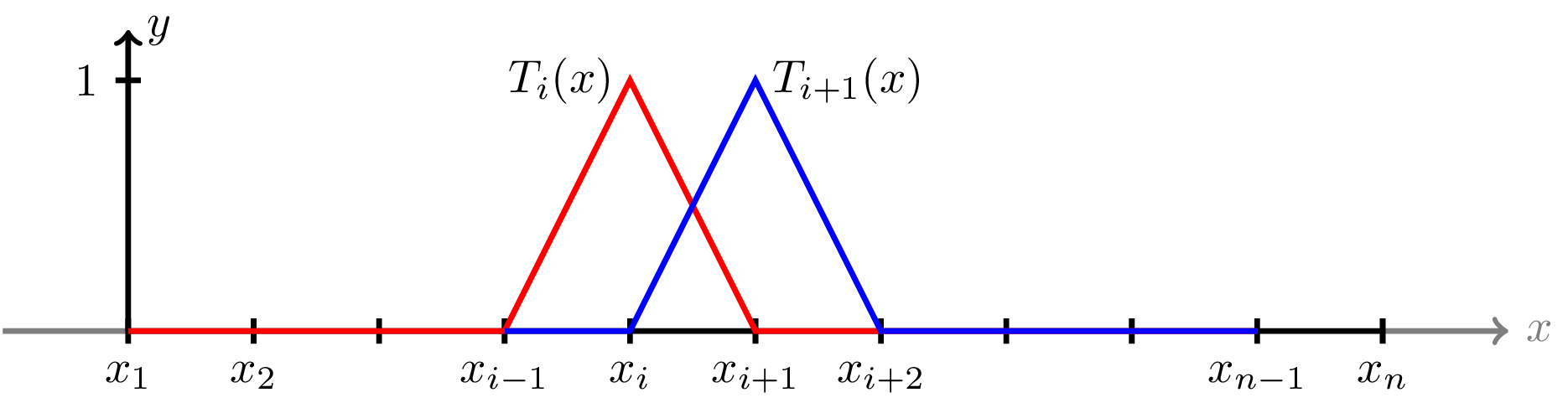
Utilizing the same basis functions for the interpolation scheme for the physics we have that
\[ p(x) = \mathbf{T}_p(x)\mathbf{p}. \]For some given values of \(p_i\) one see that the interpolation is linear on each element

Quadratic
We know continue to the concept of quadratic elements. Also here we split the domain \(\Omega = [0,L]\) into elements
The topology in this case is
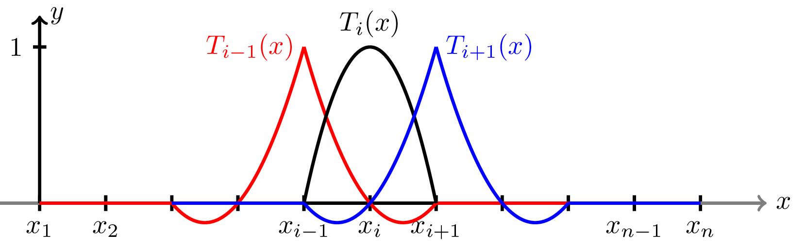
\[ \text{topology} = \begin{bmatrix} 1 & 3 & \dots & n-4 & n-2 \\ 2 & 4 & \dots & n-3 & n-1 \\ 3 & 5 & \dots & n-2 & n \end{bmatrix}. \]Note that for this case each element contains three nodes. This can be rationalized since we want quadratic elements, we must have three equations in order to find the arbitrary constants of
\[ T_{i-1}(x)x_{i-1} + T_{i}(x)x_{i} = T_{i+1}(x)x_{i+1} = ax^2 + bx + c, \quad x\in[x_{i-1}, x_{i+1}] \]Now we can set up three equations
\[ \begin{aligned} x_{i-1} &= ax_{i-1}^2 + bx_{i-1} + c\\ x_i &= ax_i^2 + bx_i + c\\ x_{i+1} &= ax_{i+1}^2 + bx_{i+1} + c. \end{aligned} \]Solving these equations one find that
\[ \begin{aligned} T_{i-1}(x) &= 2\left(\frac{x_{i}-x}{h_i}\right)\left(\frac{x_{i+1}-x}{h_i}\right)\\ T_{i}(x) &= 4\left(\frac{x-x_{i-1}}{h_i}\right)\left(\frac{x_{i+1}-x}{h_i}\right), \quad x\in[x_{i-1},x_{i+1}]\\ T_{i+1}(x) &= 2\left(\frac{x-x_{i-1}}{h_i}\right)\left(\frac{x-x_i}{h_i}\right) \end{aligned} \]Similar to the linear functions the above is only true when \(x\in[x_{i-1},x_{i+1}]\). We therefore usually denote the element interpolation as

Where \(T_i^1(x)=T_i^2(x)=T_i^3(x)=0\) when \(x\notin[x_{i-1},x_{i+1}]\). However, we can again easily generalize the definitions to hold for all \(x\) as
We can again compute the quadratic interpolation as
\[ p(x) = \mathbf{T}_p(x)\mathbf{p}. \]Now chosing the same values of \(\mathbf{p}\) as for the linear interpolation we find that 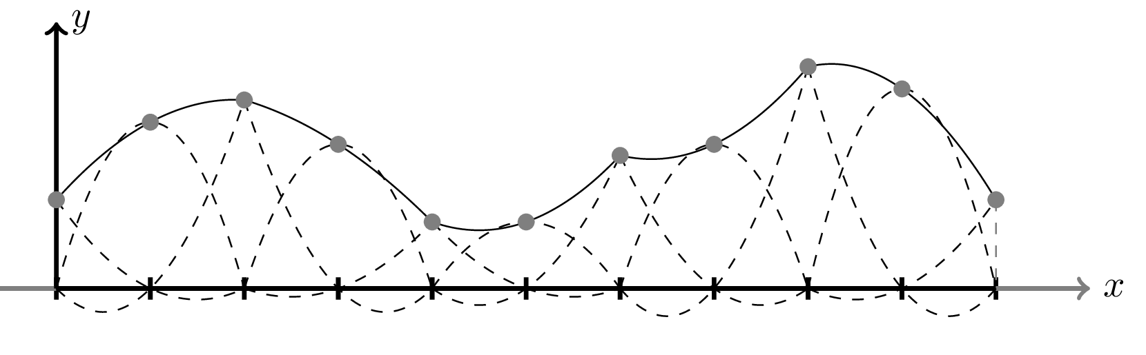
Linear vs. Quadratic interpolation
Using the same values for \(\mathbf{p}\) we can compare the results of the linear and quadratic interpolation as

Discontinuous Elements
The main idea behind discontinuous elements is to seperate the interpolation of the physics from the interpolation of the geometry. This essentially means that the interpolation nodes of the physics (\(t_i\)) will not be the same as the interpolation nodes of the geometry (\(x_i\)). What we do instead here is to introduce
Constant
The domain decomposition for constant elements look similar to that of linear continuous elements 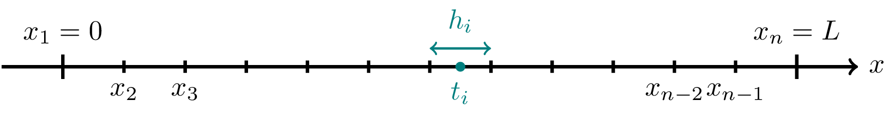
However, the difference is now that the interpolation of the physics happens only at \(t_i\) for element \(i\). This means that the topology for the physics in the case is easily written as
\[ \text{topology} = \begin{bmatrix} 1 & 2 & 3 & \dots & n-1 & n \end{bmatrix} \]As the name suggest the is constant, this simply means that
\[ T_i^1(x) = \begin{cases} 1, \quad x\in[x_i,x_{x_i}]\\0, \quad \text{otherwise}\end{cases}, \]which can be visualized as follows

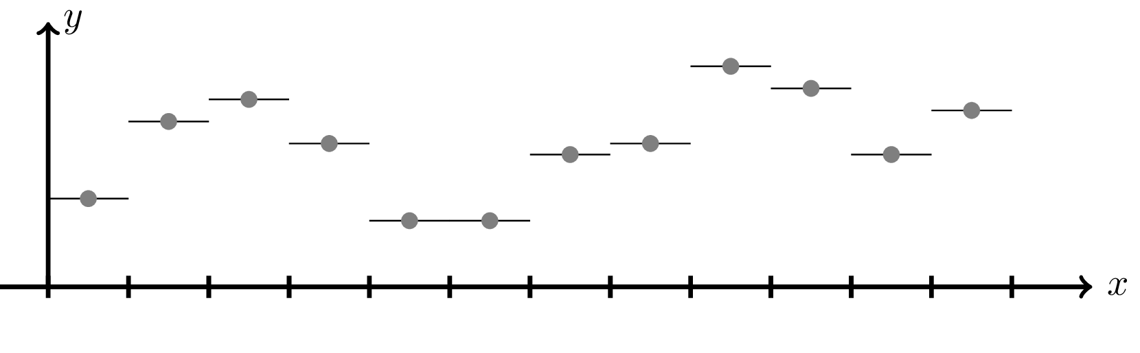
The resulting interpolation of the physics will therefore be piecewise constant as shown below
Linear
The domain decomposition for discontinuous linear elements is equivalent of that of continuous linear elements, with the difference only being the chosen interpolation nodes of the physics (\(t_i\) and \(t_{i+1}\))
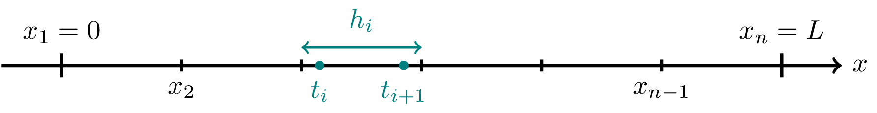
The corresponding topology of the physics is then
\[ \text{topology} = \begin{bmatrix} 1 & 3 & 5 & \dots & n-3 & n-1 \\ 2 & 4 & 6 & \dots & n-2 & n \end{bmatrix} \]The corresponding basis functions are simply just the continuous linear basis functions translated with a constant, \(\beta\), which looks as follows
\[ \begin{aligned} T_i^{\beta}(x) &= \left(\frac{x_{i+1} - x + \beta}{h_i}\right) \\ T_{i+1}^{\beta}(x) &= \left(\frac{x - x_i + \beta}{h_i}\right) \end{aligned} \]These basis functions looks as follows 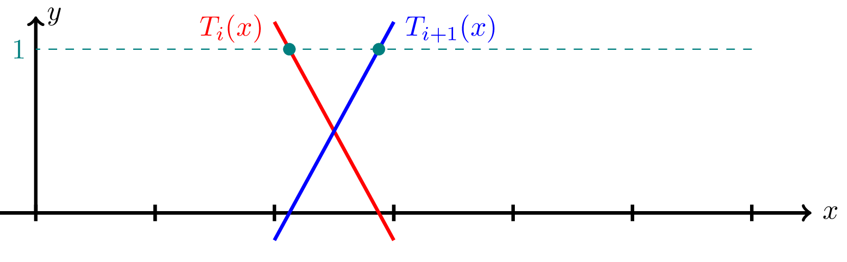
Similarily the interpolation looks as 
Quadratic
For discontinuous quadratic elements the deomain decomposition is also equivalent to continuous quadratic elements.
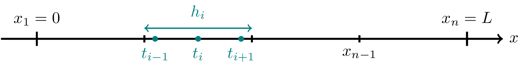
with the only difference being the interpolation nodes \(t_{i-1}\) and \(t_{i+1}\) being located inside the element. The corresponding topology matrix of the physics is
\[ \text{topology} = \begin{bmatrix} 1 & 4 & 7 & \dots & n-5 & n-2 \\ 2 & 5 & 8 & \dots & n-4 & n-1 \\ 3 & 6 & 9 & \dots & n-3 & n \end{bmatrix} \]The basis functions are also simply the continuous functions translated into the domain of the geometric element
\[ \begin{aligned} T_{i-1}^\beta(x) &= 2\left(\frac{x_{i}-x+\beta}{h_i}\right)\left(\frac{x_{i+1}-x+\beta}{h_i}\right)\\ T_{i}^\beta(x) &= 4\left(\frac{x-\beta-x_{i-1}}{h_i}\right)\left(\frac{x_{i+1}-x+\beta}{h_i}\right)\\ T_{i+1}^\beta(x) &= 2\left(\frac{x-\beta-x_{i-1}}{h_i}\right)\left(\frac{x-\beta-x_i}{h_i}\right) \end{aligned} \]which looks as 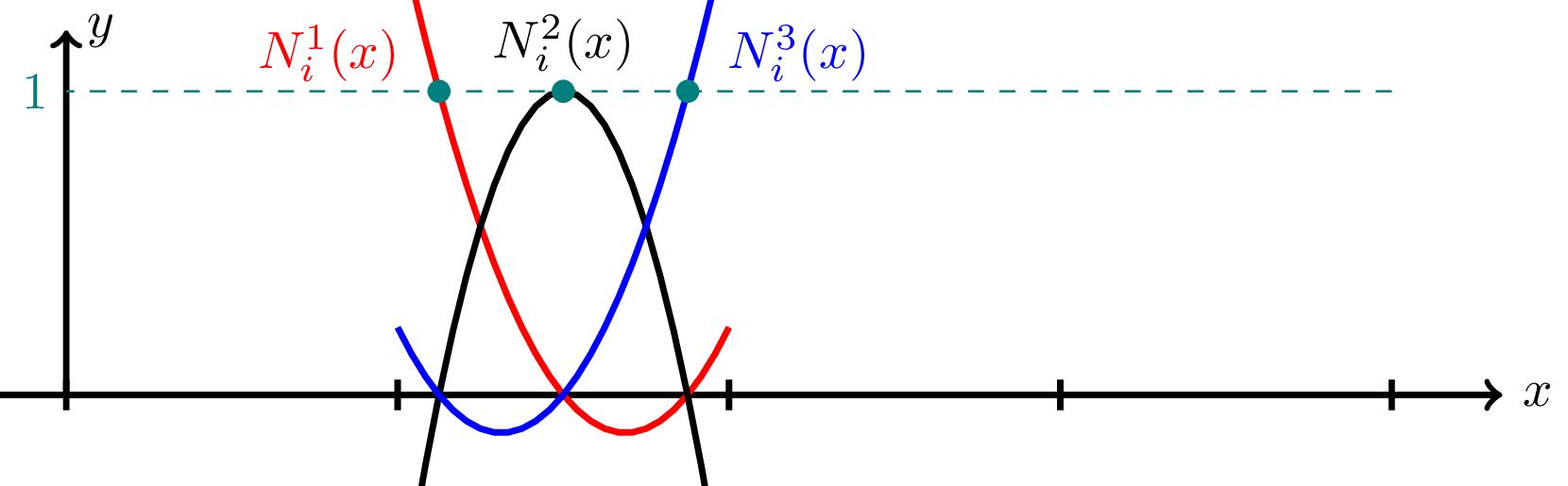
Again we can plot the interpolation as