Shape Function Derivatives

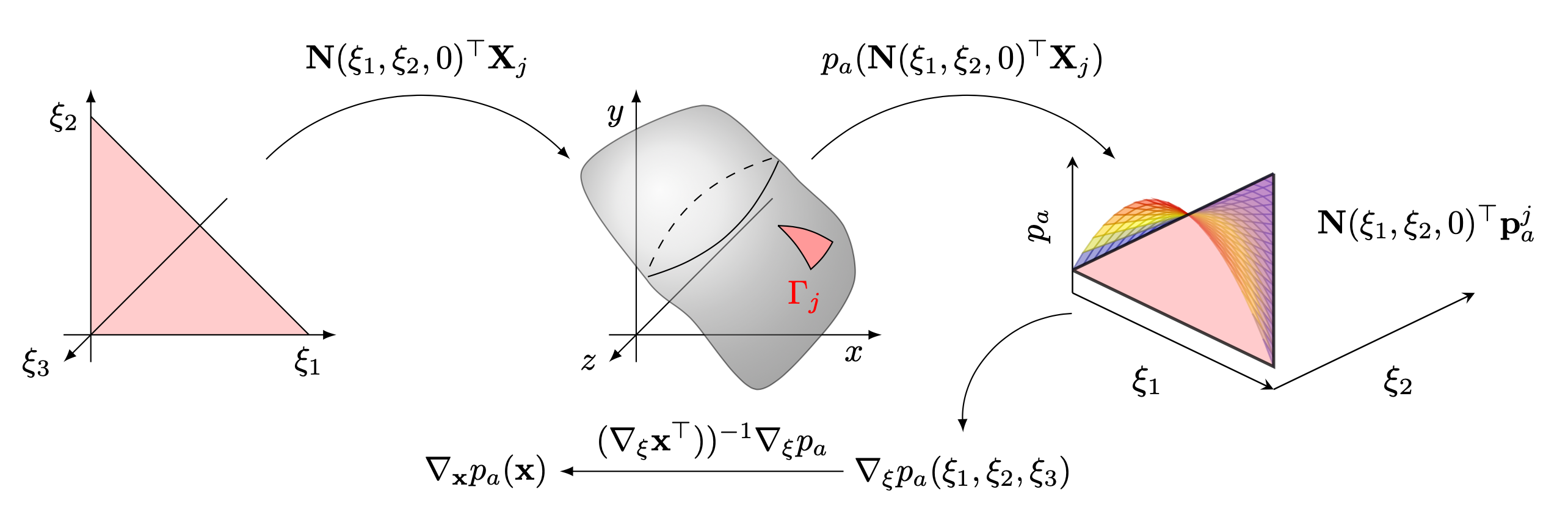
In the most basic terms the so-called shape function derivatives are simply the derivatives of the boundary element representation of the approximated functions \(p_a\), \(p_h\) and \(\mathbf{v}_v\). In order to highlight this explicitly the standard notation \(\mathbf{x} = \begin{bmatrix} x & y & z \end{bmatrix}^\top\) and \(\mathbf{\xi} = \begin{bmatrix} \xi_1 & \xi_2 & \xi_3 \end{bmatrix}^\top\) is introduced. Furthermore we will restrict the problem to exclusively look at the representation of the acoustic pressure \(p_a\). In the end it will become clear the results from this single case is immediately applicable to the thermal and viscous variables if their Boundary Element representation are chosen to be the same as the acoustic variables, which more often than not will be the case. On element \(j\) the Boundary Element representation of the interpolation is given as

\[ p_a(\mathbf{x}(\mathbf{\xi})) = p_a(\mathbf{N}(\mathbf{\xi})^\top\mathbf{X}_j) = \mathbf{N}(\mathbf{\xi})^\top \mathbf{p}_a^j, \quad \mathbf{x} \in \Gamma_j, \]

where \(\mathbf{p}_a^j\) represent the nodal acoustical pressures of element \(j\). The resulting gradient of \(p_a\) on element \(j\) is then given as

\[ \nabla_{\mathbf{\xi}}p_a(\mathbf{x}(\mathbf{\xi})) = \nabla_{\mathbf{\xi}}(\mathbf{N}(\mathbf{\xi})^\top\mathbf{p}_a^j) = (\nabla_{\mathbf{\xi}}\mathbf{N}(\mathbf{\xi})^\top)\mathbf{p}_a^j \]

since the values \(\mathbf{p}_a^j\) are constants. The last ingredient is to apply the multivariate chain rule \(\nabla_{\mathbf{\xi}}p_a = (\nabla_{\mathbf{\xi}}\mathbf{x}^\top)\nabla_\mathbf{x} p_a\) and isolate w.r.t \(\nabla_\mathbf{x}\). However, there is a slight problem in this last statement coming from the fact that the computations are based on Boundary Elements, meaning that \((\nabla_{\mathbf{\xi}}\mathbf{x}^\top)\) in theory should be a \(2\times 3\)-matrix which can not be inverted. However, it has been shown that it is enough to introduce an artificial \(\xi_3\) and assert \(\frac{\partial\mathbf{N}}{\partial \xi_3}^\top = \mathbf{0}^\top\) (with \(\mathbf{0}\) being a vector of zeros with length equal to the number of element basis functions), while substituting \(\frac{\partial\mathbf{x}}{\partial \xi_3} = \frac{\partial\mathbf{x}}{\partial \xi_1}\times \frac{\partial\mathbf{x}}{\partial \xi_2}\) (see ^[1]). The resulting expression for \(\nabla_\mathbf{x} p_a\) then becomes

\[\begin{aligned} \nabla_\mathbf{x} p_a(\mathbf{x}) = (\nabla_{\mathbf{\xi}}\mathbf{x}(\mathbf{\xi})^\top)^{-1}(\nabla_\mathbf{\xi}\mathbf{N}(\mathbf{\xi})^\top) \mathbf{p}_a^j = \begin{bmatrix} \frac{\partial x}{\partial \xi_1} & \frac{\partial y}{\partial \xi_1} & \frac{\partial z}{\partial \xi_1}\\ \frac{\partial x}{\partial \xi_2} & \frac{\partial y}{\partial \xi_2} & \frac{\partial z}{\partial \xi_2}\\ \frac{\partial x}{\partial \xi_3} & \frac{\partial y}{\partial \xi_3} & \frac{\partial z}{\partial \xi_3} \end{bmatrix} ^{-1} \begin{bmatrix} \frac{\partial\mathbf{N}}{\partial \xi_1}^\top\\ \frac{\partial\mathbf{N}}{\partial \xi_2}^\top\\ \frac{\partial\mathbf{N}}{\partial \xi_3}^\top\\ \end{bmatrix} \mathbf{p}_a^j, \quad \mathbf{x} \in \Gamma_j. \end{aligned}\]

An important aspect of the above is that the expression in front of \(\mathbf{p}_a^j\) is completely independent of the values of \(\mathbf{p}_a^j\), meaning that that if one utilizes the same discretization for all of the three modes, then the above expression can be reused for all three modes. In the case of collocation on nodes that are shared between elements the shape function derivatives is chosen to be the average of the contributions form all of the elements connected to said node.

There exist several ways of going forward at this stage. The approach taken here follows that of ^[2] which splits the gradient into its directional components. The resulting matrices in this case will have rows such that when row \(i\) is multiplied with the nodal values the result would be equal to the (averaged) shape function derivative at node \(i\). Written out this means that

\[ \frac{\partial\mathbf{p}_a}{\partial x} = \mathbf{D}_x\mathbf{p}_a, \quad \frac{\partial\mathbf{p}_a}{\partial y} = \mathbf{D}_y\mathbf{p}_a, \quad \frac{\partial\mathbf{p}_a}{\partial z} = \mathbf{D}_z\mathbf{p}_a. \]

As a final remark it should be noted that if the chosen discretization of the thermal and viscous modes are the same as for the acoustical mode then the above shape function derivative matrices can be reused to compute \(\nabla_\mathbf{x} p_h\) and \(\nabla_\mathbf{x}\cdot \mathbf{v}_v\) respectively, since this would mean that their interpolation are given as

\[ p_h(\mathbf{x}) = \mathbf{N}(\mathbf{\xi})^\top\mathbf{p}_h^j,\quad v_{x}(\mathbf{x}) = \mathbf{N}(\mathbf{\xi})^\top \mathbf{v}_{x}^j,\quad \mathbf{v}_{y}(\mathbf{x}) = \mathbf{N}(\mathbf{\xi})^\top \mathbf{v}_{y}^j,\quad \mathbf{v}_{z}(\mathbf{x}) = \mathbf{N}(\mathbf{\xi})^\top \mathbf{v}_{z}^j, \quad \mathbf{x}\in\Gamma_j, \]

resulting in the same expression as (3) with the exception of different nodal values.

References

[2]

Cutanda Henriquez, Vicente, and Peter Risby Andersen. “A Three-Dimensional Acoustic Boundary Element Method Formulation with Viscous and Thermal Losses Based on Shape Function Derivatives.” Journal of Computational Acoustics, vol. 26, no. 3, World Scientific Publishing Co. Pte Ltd, 2018, p. 1850039, doi:10.1142/S2591728518500391.

[1]	Atalla, Noureddine, and Franck Sgard. “Finite Element and Boundary Methods in Structural Acoustics and Vibration.” Finite Element and Boundary Methods in Structural Acoustics and Vibration, CRC Press, 2015, pp. 1–444, doi:10.1201/b18366.