Shape Functions

In this note we look at shape functions as a means of interpolating between nodes in a given coordinatesystem. In general the interpolation will have the form

\[ \mathbf{r}(\mathbf{\xi}) = \mathbf{M}^\top\mathbf{N}(\mathbf{\xi}), \quad \xi \in [\mathbf{a},\mathbf{b}] \]

where \(\mathbf{M}^\top = \begin{bmatrix} \mathbf{m}_1 & \dots & \mathbf{m}_n\end{bmatrix}\) is a matrix containing the interpolation nodes (\(\mathbf{m}_i\)), \(\mathbf{N}(\mathbf{\xi})\) is a vector containing the shape functions and \(\mathbf{a},\mathbf{b}\in\mathbf{R}^m\) so that \([\mathbf{a},\mathbf{b}]\) describes a hyperretangular domain in a \(m\)-dimensional space. We will in this note only consider the cases of curves (\(m=1\)) and surfaces (\(m=2\)).

Furthermore we will restrict ourselves to only talk about shape functions for curves and surfaces. The usefulness of these shape functions comes from the fact that they can be used to approximate curves and surfaces so that approximations of curve- and surface integrals can be computed easily. The reason for this focus is that only curve and surface integrals are needed for the usage of the bounary element method in two- and three-dimensional space.

Curve shape functions

We now introduce two types of shape functions for curve integrals.

Linear elements

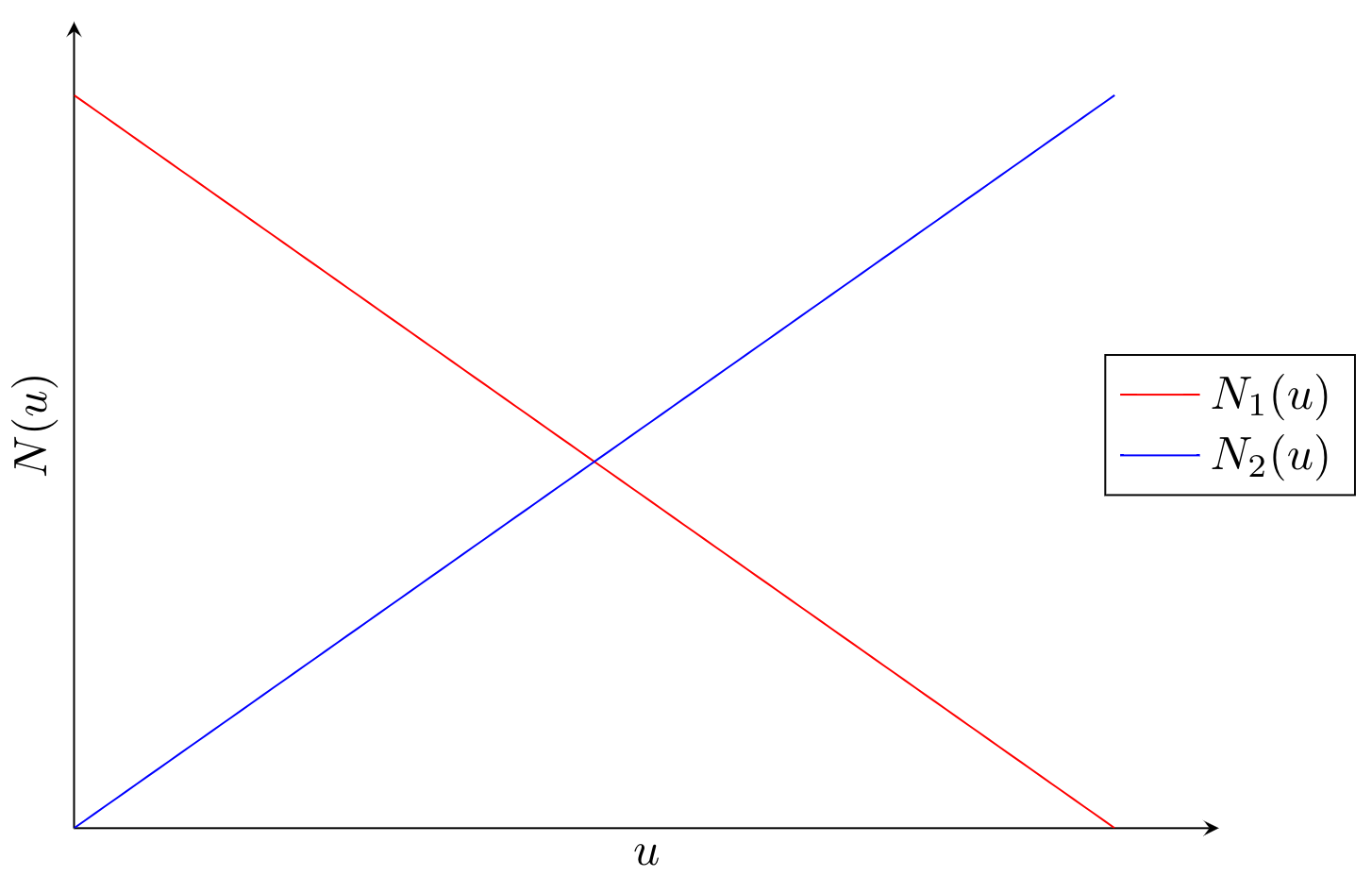
The simplest shape function for curve integrals are the linear shape function.

\[ \mathbf{N}_L(u) = \begin{bmatrix} 1 - u\\ u\end{bmatrix},\quad u \in [0,1] \]

Visually we can view the elements of \(\mathbf{N}_L(u)\) as function that are \(1\) when the other is \(0\).

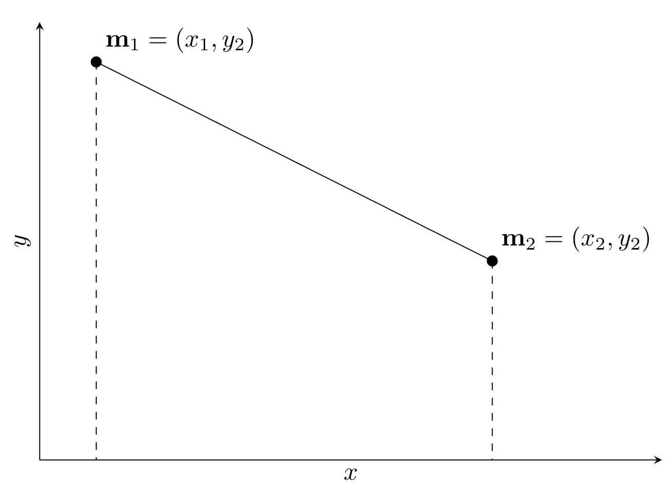
Using this shape function we can interpolate linearly between \(\mathbf{m}_1\) and \(\mathbf{m}_2\) using the parametrization

\[ \mathbf{r}_L(u) = \mathbf{M}^\top\mathbf{N}_L(u), \]

Visually this parametrization can be seen as

Now the Jacobian can we found by first computing \(\mathbf{N}_L'(u)\)

\[ \mathbf{N}_L'(u) = \begin{bmatrix} -1\\ 1\end{bmatrix},\quad u \in [0,1]. \]

Now we have that

\[ \text{Jacobi}_L(u) = \left\| \mathbf{M}^\top\mathbf{N}_L'(u)\right\|_2 = \|\mathbf{m}_2 - \mathbf{m}_1\|_2 \]

Quadratic elements

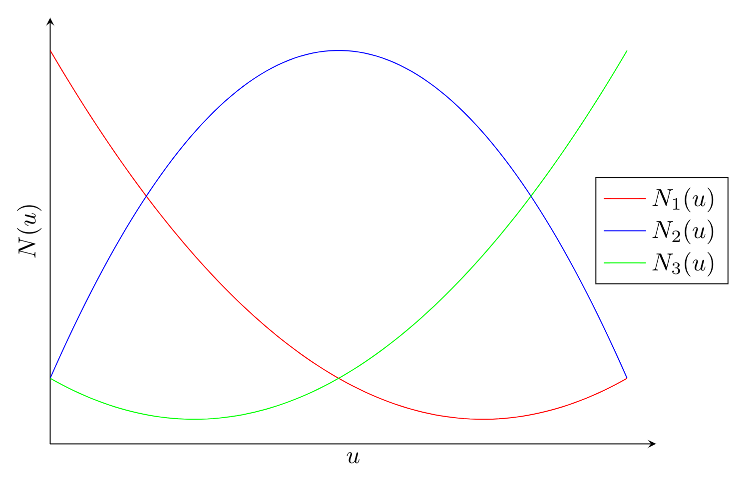
Another simple shape function is the quadratic elements defined by

\[ \mathbf{N}_Q(u) = \begin{bmatrix} \frac{1}{2}u (u - 1)\\ (1-u)(1+u)\\ \frac{1}{2}u (u + 1)\end{bmatrix}, \quad u\in[-1,1]. \]

Again we can view each element of \(\mathbf{N}_Q(u)\) as a seperate function that is equal to \(1\) when the others are \(0\)

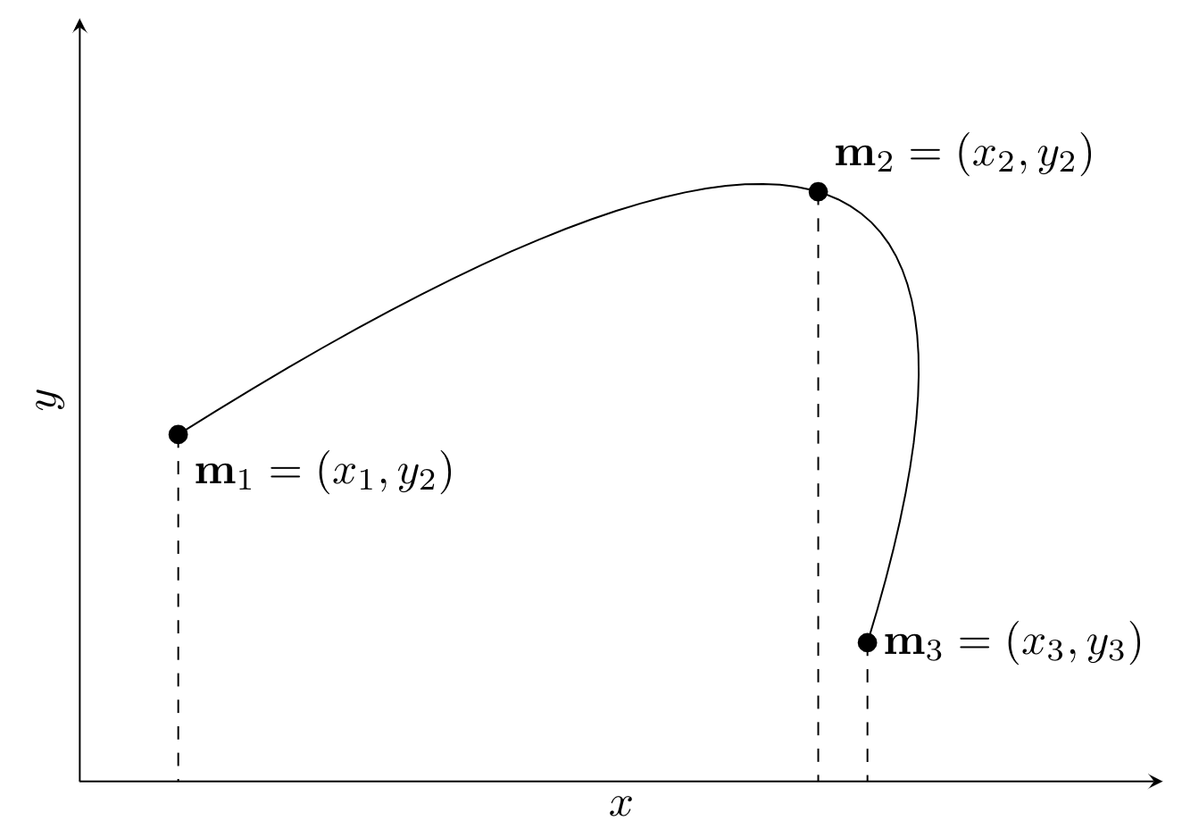
Using the quadratic shape functions we can interpolate between \(\mathbf{m}_1\), \(\mathbf{m}_2\) and \(\mathbf{m}_3\) using a quadratic as

\[ \mathbf{r}_Q(u) = \mathbf{M}^\top\mathbf{N}_Q(u). \]

Visually this interpolation can be seen as

Now the Jacobian can be computed similarily to the linear shape functions. Namely that we first compute the tagent to the shape function vector

\[ \mathbf{r}_Q'(u) = \begin{bmatrix} u - \frac{1}{2}\\ -2u \\ u + \frac{1}{2}\end{bmatrix}, \]

from which we can compute the Jacobian as

\[ \text{Jacobi}_Q(u) = \left\|\mathbf{M}^\top\mathbf{N}_Q'(u)\right\|_2 \]

Surface Shape Functions

The idea behind the surface shape functions are the exact same as for the curve shape functions. The only thing is that our parameterization now have a two-dimensional input.

Quadrilateral Shape Functions

We start by introducing the quadrilateral surface shape functions. The main reason to use this specific kind of shape function is because that they are easy to integrate, as they are defined on a rectangular domain. However the downside of the quadrilateral surface shape functions is that it is hard to efficiently create the underlying mesh.

Linear

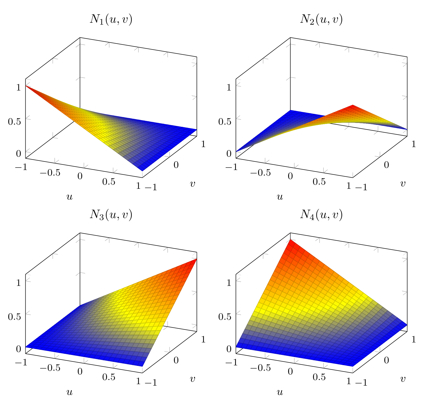
The linear surface shape functions can be described by

\[ \mathbf{N}_L(u,v) = \begin{bmatrix} \frac{1}{4}\left(1-u\right)\left(1-v\right)\\ \frac{1}{4}\left(1+u\right)\left(1-v\right)\\ \frac{1}{4}\left(1+u\right)\left(1+v\right)\\ \frac{1}{4}\left(1-u\right)\left(1+v\right) \end{bmatrix}, \quad u,v\in[-1,1]. \]

We can visually every element of the shape function by itself as

Using the shape functions it is possible to interpolate between 4 points in the \((x,y,z)\) space as. An example can be seen below.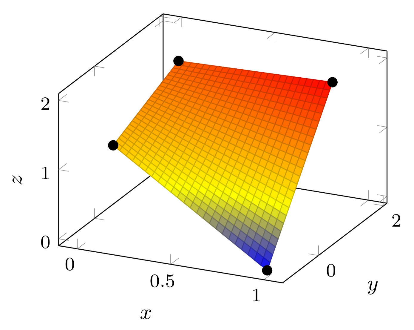

Quadratic

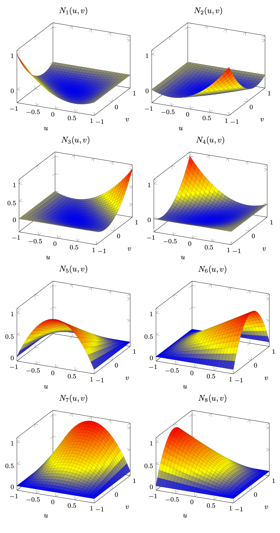
The quadratic shape functions can be described by

\[ \mathbf{N}_Q(u,v) = \begin{bmatrix} \frac{1}{4}\left(1-u\right)\left(v-1\right)\left(u+v+1\right)\\ \frac{1}{4}\left(1+u\right)\left(v-1\right)\left(v-u+1\right)\\ \frac{1}{4}\left(1+u\right)\left(1+v\right)\left(u+v-1\right)\\ \frac{1}{4}\left(u-1\right)\left(1+v\right)\left(u-v+1\right)\\ \frac{1}{2}\left(1-v\right)\left(1-u^2\right)\\ \frac{1}{2}\left(1+u\right)\left(1-v^2\right)\\ \frac{1}{2}\left(1+v\right)\left(1-u^2\right)\\ \frac{1}{2}\left(1-u\right)\left(1-v^2\right) \end{bmatrix}, \quad u,v\in[-1,1]. \]

Again we can visualize every element by itself.

Using the shape functions it is possible to interpolate between 8 points in the \((x,y,z)\) space as. An example can be seen below.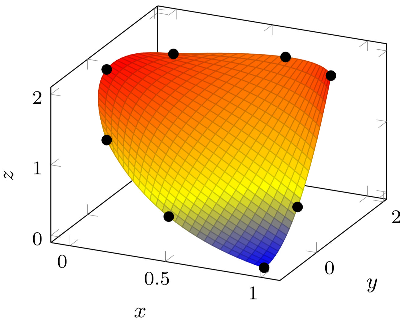

Triangular Shape Functions

We now briefly introduce triangular surface shape functions. In constrast to the quadrilateral surface shape functions there exist many efficient ways of computing these triangular meshes. However the integration of these shape functions requires an extra step, since they are defined on a triangular domain instead of the usual rectangular domain.

Linear

The linear triangular surface shape functions are defined as follows

\[ \mathbf{N}_L(u,v) = \begin{bmatrix}1-u-v\\u\\v\end{bmatrix}, \quad u\in[0,1],v\in[0,1-u]. \]

Visually we can see them as.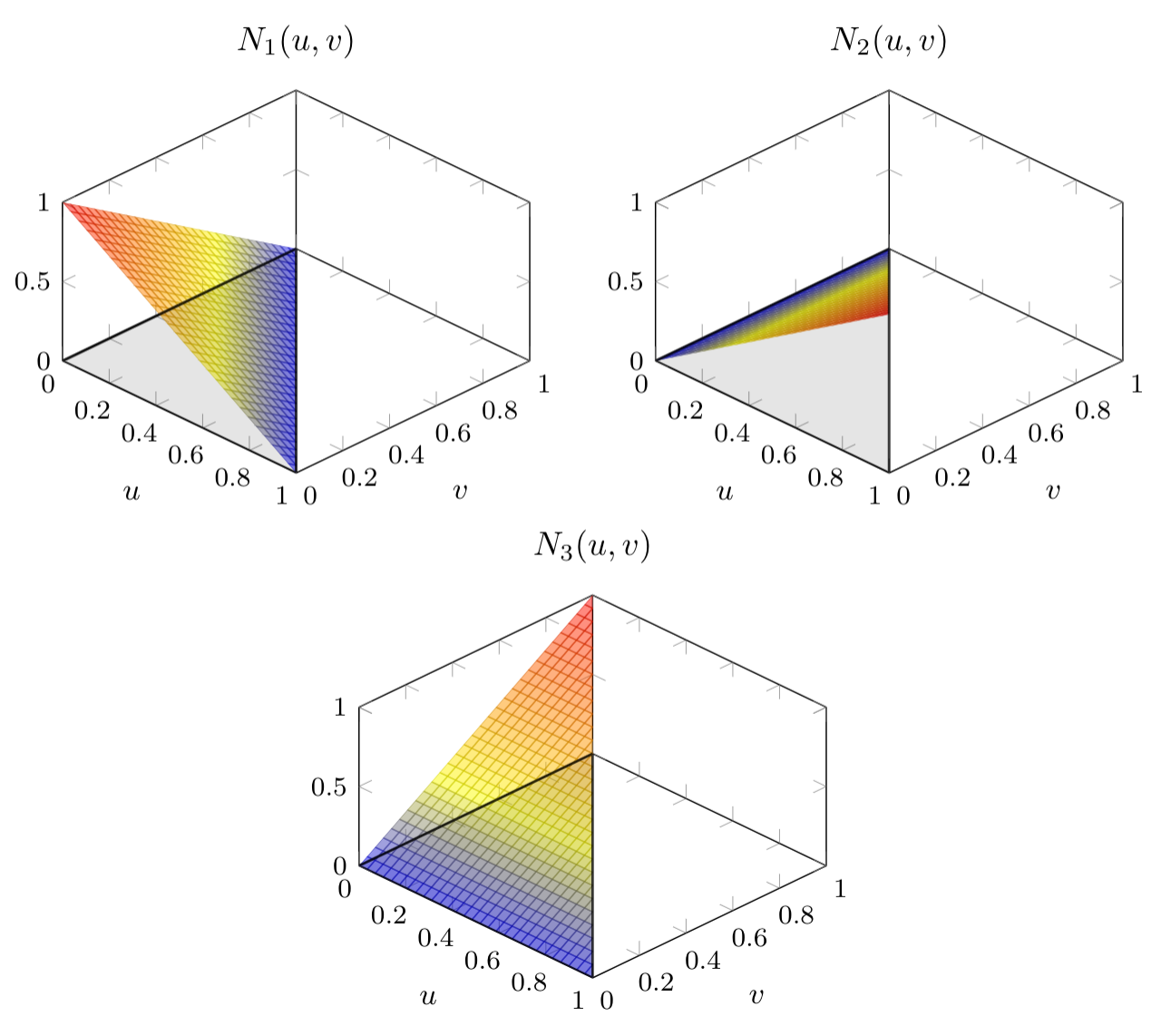

Quadratic

Now the quadratic triangular shape functions are defined as follows

\[ \mathbf{N}_Q(u,v) = \begin{bmatrix}(1-u-v)(1-2u-2v)\\u(2u-1)\\v(2v-1)\\4u(1-u-v)\\4uv\\4v(1-u-v)\end{bmatrix}, \quad u\in[0,1],v\in[0,1-u]. \]

Plotting every element for itself we see that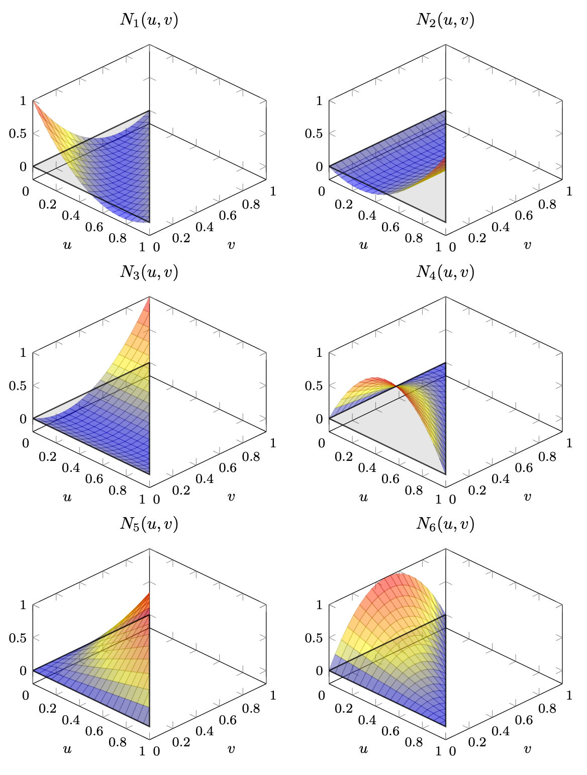

Quadrature On Triangular Shape Functions

In order for us to integrate over the triangular domains using a quadrature scheme we need to transform the coordinate into a rectangular domain. This can be done using the following transformation

\[ \begin{bmatrix}u \\ v\end{bmatrix} = \begin{bmatrix} \xi\\ \eta(1-\xi)\end{bmatrix}, \xi,\eta \in [0,1]. \]

The Jacobian in this case can be computed analytically as

\[ \text{Jacobi}_T(\xi,\eta) = \left|\det\left(\begin{bmatrix}1 & 0\\ -\eta & 1-\xi\end{bmatrix}\right)\right| = 1-\xi. \]

Note that since \(\xi \in [0,1]\) we can remove the absolute value. We can transform the integral as

\[\begin{aligned} \int_0^{1-u}\int_0^1 &f(r(u,v))\text{Jacobi}_r(u,v)\ \mathrm{d}u\mathrm{d}v = \\ &\int_0^1\int_0^1 f(r(\xi,\eta(1-\xi))\text{Jacobi}_r(\xi,\eta(1-\xi))\text{Jacobi}_T(\xi,\eta) \ \mathrm{d}\xi\mathrm{d}\eta = \\ &\int_0^1\int_0^1 f(r(\xi,\eta(1-\xi))\text{Jacobi}_r(\xi,\eta(1-\xi))(1 - \xi)\ \mathrm{d}\xi\mathrm{d}\eta. \end{aligned}\]

Given that the above integral is now defined on a rectangular domain it can be approximated using a suitable quadrature scheme in both the \(\xi\) and \(\eta\) direction.

The result is therefore that

\[\begin{aligned} \int_0^{1-u}\int_0^1 &f(r(u,v))\text{Jacobi}_r(u,v)\ \mathrm{d}u\mathrm{d}v \approx \\ &\sum_{i=1}^{l_1}\sum_{j=1}^{l_2} w_iw_jf(r(\xi_i,\eta_j(1-\xi_i))\text{Jacobi}_r(\xi_i,\eta_j(1-\xi_i))(1 - \xi_i) \end{aligned}\]