The Finite Element Method
The aim of the Finite Element Method (FEM) is to solve (or more precisely approximate the solution of) a Partial Differential Equation (PDE) using a computer. In general the solution to a PDE is a function. Unfortunately it is computationally intractable to task a computer with finding this underlying function. The idea to resolve this issue is to parametrize a family of functions with the aim of computing the parameters through solving linear system of equations. There are a plethora of ways to get to such a linear system of equations, with the most common being the so-called Galerkin approach.
Getting the computer to understand functions
In the most basic terms, computers are only capable of understanding numbers, which means that they are inherently unable to solve equations where the unknowns are functions. This is a problem when trying to solve differential equations. To solve this problem, the functions are instead approximated using parameterizations for which the coefficients (numbers) are unknown. Intuitively, these numbers are exactly what the computer is asked to find. For element methods, this parameterization is chosen to be the simplest possible: A linear combination of functions
\[ p(\mathbf{x}) \approx \mathbf{T}(\mathbf{x})\mathbf{p} = \begin{bmatrix} T_1(\mathbf{x}) & T_2(\mathbf{x}) & \dots & T_n(\mathbf{x}) \end{bmatrix} \begin{bmatrix} p_1 \\ p_2 \\ \vdots \\ p_n \end{bmatrix}. \]where \(p\) is the unknown function being approximated. Note that the linearity is with respect to the unknown parameters \(\mathbf{p}\), but not necessarily in the known basis functions \(\mathbf{T}(\mathbf{x})\).
One might ask: How does the above relate to The Finite Element Method? The answer is that the functions \(\mathbf{T}_i\) are chosen to be simpler functions with support equal to only a few subdomains of the original domain. These subdomains are commonly referred to as elements. In the case of 1D line elements are used.
The Finite Element Method for the Helmholtz equation
In acoustics we are often interested in solving Helmholtz equation given as
\[ \Delta p(\mathbf{x}) + k^2p(\mathbf{x}) = 0, \mathbf{x} \in \Omega \]where \(k\) is most often referred to as the wavenumber.
At its current form there is a strict constraint on the order of the numerical solution of \(p(\mathbf{x})\), as the 2nd derivative of the functions \(\mathbf{T}(\mathbf{x})\) can not be zero. This constraint can be relieved using the so-called weak formulation. In order to do so we multiply the Helmholtz equation with a so-called test function \(\phi\) following by the integration over the domain \(\Omega\)
\[ \int_\Omega \phi(\mathbf{x})\left(\Delta p(\mathbf{x}) + k^2p(\mathbf{x})\right)\ \mathrm{d}\mathbf{x} = 0. \]Utilizing integration by parts on the term including the Laplacian we can move derivatives from \(p(\mathbf{x})\) onto \(\phi(\mathbf{x})\) as
\[ \int_\Omega \left(\nabla\phi(x)\right)^\top\nabla p(x)\ \mathrm{d}\mathbf{x} - k^2\int_\Omega\phi(x)p(x)\ \mathrm{d}\mathbf{x} - \int_{\partial\Omega}\phi(x)\frac{\partial p}{\partial n}(x)\ \mathrm{d}\mathbf{x} = 0. \]In the above the constraint on the smoothness of \(p(\mathbf{x})\) has been reduced to first order. Furthermore the last term
\[ \int_{\partial\Omega}\phi(x)\frac{\partial p}{\partial n}(x)\ \mathrm{d}\mathbf{x}, \]can be used to include the boundary conditions into the equation. For simplification purposes we will in the following assume that the above is equal to zero. As such we have that
\[ 0 = \int_\Omega \left(\nabla\phi(x)\right)^\top\nabla p(x)\ \mathrm{d}\mathbf{x} - k^2\int_\Omega\phi(x)p(x)\ \mathrm{d}\mathbf{x} . \]We will now use the Galerkin approach to discretize the above equation. Note that Galerkin simply refers to the approach where \(\phi(\mathbf{x})\) and \(p(\mathbf{x})\) is discretized using the same basis functions (\(\mathbf{T}(\mathbf{x})\)). In short this means that we introduce
\[ p(\mathbf{x}) \approx \mathbf{T}(\mathbf{x})\mathbf{p}, \quad \phi(\mathbf{x}) \approx \mathbf{a}^\top\mathbf{T}(\mathbf{x})^\top, \]where \(\mathbf{a} \in \mathbf{C}^n\) is a set of arbitrary coefficients that parametrized a whole family of test functions and \(\mathbf{p}\in\mathbb{C}^n\) is the coefficients that we aim to find. Inserting the approximations it follows that
\[ \begin{aligned} 0 &= \int_\Omega \left(\nabla\phi(x)\right)^\top\nabla p(x)\ \mathrm{d}\mathbf{x} - k^2\int_\Omega\phi(x)p(x)\ \mathrm{d}\mathbf{x}\\ &\approx \int_\Omega\mathbf{a}^\top(\nabla\mathbf{T}(\mathbf{x}))^\top\nabla\mathbf{T}(\mathbf{x})\mathbf{p}\ \mathrm{d}\mathbf{x} - k^2\int_\Omega\mathbf{a}^\top \mathbf{T}(\mathbf{x})^\top\mathbf{T}(\mathbf{x})\mathbf{p}\ \mathrm{d}\mathbf{x}\\ &= \mathbf{a}^\top\left(\int_\Omega(\nabla\mathbf{T}(\mathbf{x}))^\top\nabla\mathbf{T}(\mathbf{x})\ \mathrm{d}\mathbf{x}\right)\mathbf{p} - k^2\mathbf{a}^\top \left(\int_\Omega \mathbf{T}(\mathbf{x})^\top\mathbf{T}(\mathbf{x})\ \mathrm{d}\mathbf{x}\right)\mathbf{p}\\ &= \mathbf{a}^\top\left(\int_\Omega(\nabla\mathbf{T}(\mathbf{x}))^\top\nabla\mathbf{T}(\mathbf{x})\ \mathrm{d}\mathbf{x} - k^2\int_\Omega \mathbf{T}(\mathbf{x})^\top\mathbf{T}(\mathbf{x})\ \mathrm{d}\mathbf{x}\right)\mathbf{p}.\\ \end{aligned} \]We can make the above the equality hold for all possible test functions, i.e. for all \(\mathbf{a} \in \mathbb{C}^n\), if we find \(\mathbf{p}\) such that
\[ \left(\int_\Omega(\nabla\mathbf{T}(\mathbf{x}))^\top\nabla\mathbf{T}(\mathbf{x})\ \mathrm{d}\mathbf{x} - k^2\int_\Omega \mathbf{T}(\mathbf{x})^\top\mathbf{T}(\mathbf{x})\ \mathrm{d}\mathbf{x}\right)\mathbf{p} = \mathbf{0}. \]This is exactly what we do in Finite Element computations. As a shorthand the above can be written as
\[ \left(\mathbf{K} - k^2\mathbf{M}\right)\mathbf{p} = \mathbf{0}, \]where \(\mathbf{K}\) is referred to as the stiffness matrix and \(\mathbf{M}\) as the mass matrix. In literature the equation can also be found as
\[ \left(c^2\mathbf{K} - \omega^2\mathbf{M}\right)\mathbf{p} = \mathbf{0}, \]where \(c\) is the propagation speed and \(\omega\) is the angular frequency.
What is an element?
A key insight is that the element serves two purposes: It represents a subdomain of the original domain (also referred to as the geometry) while also describing parts of the unknown function(s) of interest. In the general this subdomain is described by a parameterization, i.e. the element, as
\[ \mathbf{x}^e(\mathbf{u}) = \mathbf{X}^e\mathbf{N}^e(\mathbf{u}) \in \Omega^e, \quad \forall \mathbf{u} \in \mathcal{L}^e, \]where the superscript \(e\) denotes the element number, \(\mathbf{X}^e\) is a matrix with columns equal to the interpolation nodes of the geometry, \(\mathbf{N}^e(\mathbf{u})\) are the so-called shape functions, \(\Omega^e\) is the element in global coordinates and \(\mathcal{L}^e\) are the local coordinates. In addition to the geometric interpolation of each element, we need to further define interpolations of the unknown functions, which in acoustics is usually taken as the pressure \(p(\mathbf{x})\). On element \(e\) this interpolation can be done as
\[ p(\mathbf{x}^e(\mathbf{u})) = \mathbf{T}(\mathbf{x}^e(\mathbf{u}))\mathbf{p} = \underbrace{\mathbf{T}(\mathbf{x}(\mathbf{u}))(\mathbf{L}^e)^\top}_{\mathbf{T}^e(\mathbf{u})}\underbrace{\mathbf{L}^e\mathbf{p}}_{\mathbf{p}^e} = \mathbf{T}^e(u)\mathbf{p}^e, \quad \mathbf{u} \in \mathcal{L}^e \]where \(\mathbf{L}^e\) is a permutation-like matrix that extracts the relevant values of \(\mathbf{p}\) and relevant functions of \(\mathbf{T}(\mathbf{x})\) and orders such that they correspond to the local values \(\mathbf{p}^e\) and local basis functions of \(\mathbf{T}^e(\mathbf{u})\).
For examples of \(\mathbf{N}^e(\mathbf{u})\), \(\mathbf{T}^e(\mathbf{u})\) and \(\mathbf{L}_e\) see below.
Example: (Linear triangular elements) 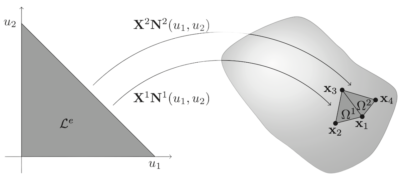
The linear shape functions for a triangular element can have the form
\[ \mathbf{N}^e(u_1,u_2) = \begin{bmatrix} 1 - u_1 - u_2 \\ u_1 \\ u_2 \end{bmatrix}, \quad u_1\in[0, 1],\ u_2\in[0, 1-u_1]. \]The choice in the wording can is because the ordering of the columns of \(\mathbf{X}^e\) can change the ordering rows of \(\mathbf{N}^e(\mathbf{u})\) or vice versa. This is something that one should keep in mind in practice when using different mesh file formats. Taking the second element of Figure above as an example, it could be that
\[ \mathbf{X}^2 = \begin{bmatrix} \mathbf{x}_3 & \mathbf{x}_1 & \mathbf{x}_4 \end{bmatrix}. \]Note that extending the geometric interpolation to higher orders is as simple as adding more rows/functions to \(\mathbf{N}^e(u_1,u_2)\) as well as more columns/points to \(\mathbf{X}^e\).
Example: (Basis functions for continuous linear interpolation) 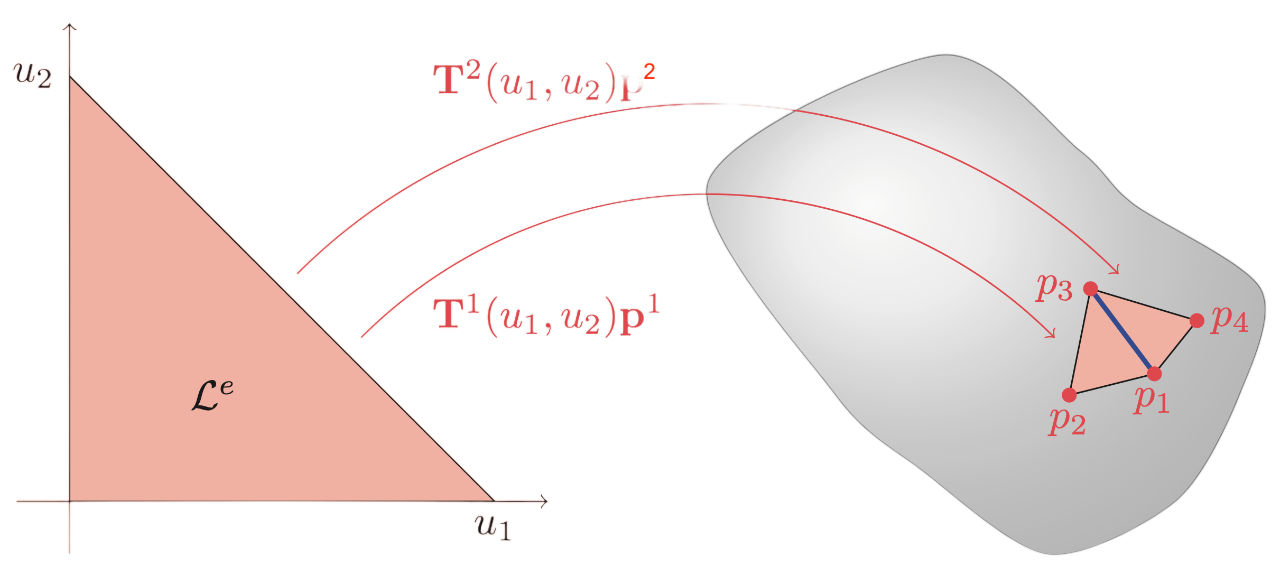
Continuous linear basis functions on triangular elements are similar to shape functions for a linear triangular element and differ only in the fact that it is the transpose.
\[ \mathbf{T}^e_\text{continuous}(u_1,u_2) = \begin{bmatrix} 1 - u_1 - u_2 & u_1 & u_2 \end{bmatrix}, \quad u_1\in[0, 1],\ u_2\in[0, 1-u_1], \]where the subscript "continuous" is only there to highlight that it is a continuous formulation. Again, the ordering of the columns of the row vector depends on the ordering of the element corners.
Example: (Basis functions for discontinuous linear interpolation) 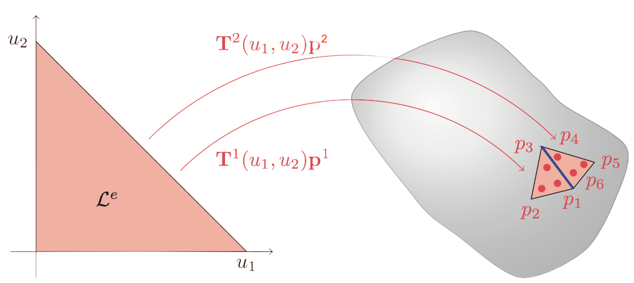
The discontinuous linear interpolation is simply a scaled continuous formulation
\[ \mathbf{T}^e_\text{discontinuous}(u_1,u_2) = \mathbf{T}^e_\text{continuous}\left(\frac{u_1 - \beta}{1-3\beta},\frac{u_2 - \beta}{1 - 3\beta}\right), \]where \(\beta \in \left[0,\frac{1}{2}\right[\) is a scalar representing the location of the interpolation nodes in the local \(\mathcal{L}^e\) coordinates.
Example: (Element Localization Matrix) For a continuous linear element \(e\) all three corners correspond to a value of the global vector \(\mathbf{p}\). For example, the second element in continuous plot has local corner values given by \(\mathbf{p}^2 = \begin{bmatrix}p_3 & p_1 & p_4 \end{bmatrix}^\top\). This element would have \(\mathbf{L}^e\) given as
\[ \mathbf{L}^2 = \begin{bmatrix} 0 & 0 & 1 & 0 & \dots & 0\\ 1 & 0 & 0 & 0 & \dots & 0\\ 0 & 0 & 0 & 1 & \dots & 0 \end{bmatrix}, \]so that \(\mathbf{p}^2 = \mathbf{L}^2\mathbf{p}\). Note that \(\mathbf{L}^e\) is only an artifact of the mathematical description. Any reasonable implementation should use indexing instead of multiplication with \(\mathbf{L}^e\). In the case of the discontinuous description the same element in discontinuous plot would have \(\mathbf{p}^2 = \begin{bmatrix}p_4 & p_5 & p_6\end{bmatrix}^\top\) meaning that
\[ \mathbf{L}^2 = \begin{bmatrix} 0 & 0 & 0 & 1 & 0 & 0 & 0 & \dots & 0\\ 0 & 0 & 0 & 0 & 1 & 0 & 0 & \dots & 0\\ 0 & 0 & 0 & 0 & 0 & 1 & 0 & \dots & 0 \end{bmatrix}. \]Note here that the discontinuous nature result in \(\mathbf{L}^e\) simply picks out three consecutive values.
Computing the stiffness and mass matrices
Using the element description of both the geometry and the pressure function the mass matrix can be computed as follows
\[ \begin{aligned} \mathbf{M} &= \int_\Omega \mathbf{T}(\mathbf{x})^\top\mathbf{T}(\mathbf{x})\ \mathrm{d}\mathbf{x} \\ &\approx \sum_{e=1}^N\int_{\Omega^e} \mathbf{L}_e^\top\mathbf{L}_e\mathbf{T}(\mathbf{x})^\top\mathbf{T}(\mathbf{x})\mathbf{L}_e^\top\mathbf{L}_e\ \mathrm{d}\mathbf{x} \\ &= \sum_{e=1}^N \mathbf{L}_e^\top\left(\int_{\mathcal{L}^e}\mathbf{T}^e(\mathbf{u})^\top\mathbf{T}^e(\mathbf{u})\text{jacobian}(\Omega^e,\mathbf{u})\ \mathrm{d}\mathbf{u}\right)\mathbf{L}_e \\ &= \sum_{e=1}^N \mathbf{L}_e^\top\left(\underbrace{\sum_{i=1}^{Q} w_i\mathbf{T}^e(\mathbf{u}_i)^\top\mathbf{T}^e(\mathbf{u}_i)\text{jacobian}(\Omega^e,\mathbf{u}_i)}_{\mathbf{M}_e}\right)\mathbf{L}_e, \end{aligned} \]where jacobian(\(\Omega^e,\mathbf{u}\)) is a function that describes the distortion from the local coordinates \(\mathcal{L}^e\) onto the global element \(\Omega^e\). This distortion represent length, area, or volume depending on the dimensionality of the problem. Note that if the elements are the same size then \(\mathbf{M}^e\) is constant with respect to each element (this is the case in the code below).
The stiffness matrix is computed similarly but with a difference in the fact that the gradient must have its coordinates changed from global to local. Using the chain rule it follows that
\[ \nabla_u p(\mathbf{x}(\mathbf{u})) = \mathbf{J}(\mathbf{u})\nabla_\mathbf{x} p(\mathbf{x}(\mathbf{u})), \]from which we can isolate the global gradient as
\[ \nabla_\mathbf{x} p(\mathbf{x}(\mathbf{u})) = \mathbf{J}(\mathbf{u})^{-1}\nabla_u p(\mathbf{x}(\mathbf{u})). \]Putting the things together the stiffness matrix can therefore be computed as
\[ \begin{aligned} \mathbf{K} &= \int_\Omega (\nabla\mathbf{T}(\mathbf{x}))^\top\nabla\mathbf{T}(\mathbf{x})\ \mathrm{d}\mathbf{x} \\ &= \sum_{e=1}^N\int_{\Omega^e} \mathbf{L}_e^\top\mathbf{L}_e(\nabla_\mathbf{x}\mathbf{T}(\mathbf{x}))^\top\nabla_\mathbf{x}\mathbf{T}(\mathbf{x})\mathbf{L}_e^\top\mathbf{L}_e\ \mathrm{d}\mathbf{x} \\ &= \sum_{e=1}^N\mathbf{L}_e^\top\left(\int_{\mathcal{L}^e} (\nabla_\mathbf{x}\mathbf{T}^e(\mathbf{u}))^\top\nabla_\mathbf{x}\mathbf{T}^e(\mathbf{u})\text{jacobian}(\Omega^e,\mathbf{u})\ \mathrm{d}\mathbf{u}\right)\mathbf{L}_e \\ &= \sum_{e=1}^N\mathbf{L}_e^\top\left(\int_{\mathcal{L}^e} (\nabla_\mathbf{u}\mathbf{T}^e(\mathbf{u}))^\top\mathbf{J}(\mathbf{u})^{-1}\left(\mathbf{J}(\mathbf{u})^\top\right)^{-1}\nabla_\mathbf{u}\mathbf{T}^e(\mathbf{u})\text{jacobian}(\Omega^e,\mathbf{u})\ \mathrm{d}\mathbf{u} \right)\mathbf{L}_e\\ &= \sum_{e=1}^N\mathbf{L}_e^\top\left(\underbrace{\sum_{i=1}^{Q} (\nabla_\mathbf{u}\mathbf{T}^e(\mathbf{u}_i))^\top\mathbf{J}(\mathbf{u}_i)^{-1}\left(\mathbf{J}(\mathbf{u}_i)^\top\right)^{-1}\nabla_\mathbf{u}\mathbf{T}^e(\mathbf{u}_i)\text{jacobian}(\Omega^e,\mathbf{u}_i)}_{\mathbf{K}_e} \right)\mathbf{L}_e. \end{aligned} \]In the following code we implement three different ways of assembling the mass and stiffness matrices. Note that two first implementations are only for educational purposes as they're both based on dense matrices.
### Importing relevant packages
using ForwardDiff
using SparseArrays
using LinearAlgebra
using BenchmarkTools
using FastGaussQuadrature
## Defining geometry.
# Models Impedance Tube of 10cm diameter and 1m in length (used later)
D = 0.1             # 100 mm diameter
L = 10*D            # Length of the cavity
ne = 600            # Number of quadratic elements
nnt = 2*ne+1        # Total number of nodes
h = L/ne            # Length of the elements
x = Vector(0:h/2:L) # Coordinates table

## Computing the element matrices
# Defining local basis functions (and gradient using ForwardDiff - This is inefficient but easy)
Tᵉ(u)  = [u .* (u .- 1)/2; 1 .- u .^2; u .* (u .+ 1)/2]'
∇Tᵉ(u) = hcat(ForwardDiff.derivative.(Tᵉ,u)...)
# Every element is the same, so the Jacobian does not depend on the element in this case.
# Furthermore we map from [-1,1] onto [x_i,x_{i+1}]. Meaning from length 2 to length h.
jacobian(u) = h/2
# In the 1D case the Jacobian function and matrix are equal. This is not true in higher dimensions.
J(u) = h/2
# Defining the local element matrices. Since the elements are the same size its constant.
Q = 3  # Number of Gaussian points used in the integration.
u,w = gausslegendre(Q)
Me = sum(i -> w[i]*Tᵉ(u[i])'*Tᵉ(u[i])*jacobian(u[i]),1:Q)
Ke = sum(i -> w[i]*∇Tᵉ(u[i])'*J(u[i])^(-1)*J(u[i])^(-1)*∇Tᵉ(u[i])*jacobian(u[i]),1:Q)

## Assembly 1: Simple (using the element localization matrices. Never do this!)
function assembly1(Me,Ke,nnt,ne)
    K = zeros(nnt,nnt)  # Dense matrix! Not ideal!
    M = zeros(nnt,nnt)  # Dense matrix! Not ideal!
    for ie = 1:ne
        Le = zeros(3,nnt)
        Le[:,ie*2-1:ie*2+1] = Diagonal(ones(3))

        K += Le'*Ke*Le
        M += Le'*Me*Le
    end
    return K,M
end
@btime K,M = assembly1(Me,Ke,nnt,ne)

## Assembly 2: Intermediate (using indexing instead of the element localization matrices)
function assembly2(Me,Ke,nnt,ne)
    K = zeros(nnt,nnt)  # Dense matrix! Not ideal!
    M = zeros(nnt,nnt)  # Dense matrix! Not ideal!
    for ie = 1:ne
        K[ie*2-1:ie*2+1,ie*2-1:ie*2+1] += Ke
        M[ie*2-1:ie*2+1,ie*2-1:ie*2+1] += Me
    end
    return K,M
end
@btime K,M = assembly2(Me,Ke,nnt,ne) # Note that the matrices are here still dense.

## Assembly 3: Advanced (Sparse assembly using the compact support of the elements.)
function assembly3(Me,Ke,nnt,ne)
    I = zeros(Int64,4nnt-3)
    J = zeros(Int64,4nnt-3)
    Kd = zeros(ComplexF64,length(I))
    Md = zeros(ComplexF64,length(I))
    for ie=1:ne
        for i = 1:3
            I[(8*(ie-1)+1 + 3*(i-1)):(8*(ie-1) + 3*i)]  .= ie*2-1:ie*2-1+2
            J[(8*(ie-1)+1 + 3*(i-1)):(8*(ie-1) + 3*i)]  .= (ie-1)*2 + i
            Kd[(8*(ie-1)+1 + 3*(i-1)):(8*(ie-1) + 3*i)] += Ke[:,i]
            Md[(8*(ie-1)+1 + 3*(i-1)):(8*(ie-1) + 3*i)] += Me[:,i]
        end
    end
    K = sparse(I,J,Kd)
    M = sparse(I,J,Md)
    return K,M
end
@btime K,M = assembly3(Me,Ke,nnt,ne)
6.298 s (9005 allocations: 25.86 GiB)
509.166 μs (2405 allocations: 22.30 MiB)
251.834 μs (10837 allocations: 1.76 MiB)
Example: Impedance Tube
Analytical Expressions
The procedure used in an impedance tube to measure the surface impedance and absorption coefficient of an acoustic material. A loudspeaker is installed at one end (\(x = L\)) and an acoustic material of thickness \(h\) and surface impedance \(\hat{Z}\) is bonded onto the other rigid and impervious end (\(x = 0\)). Below the cut-off frequency of the tube, only plane waves propagate and the problem is amenable to a one-dimensional analysis.
In this case the surface impedance of the material can be obtained from the measurement of the transfer function \(\hat{H}_{12} = \hat{P}_2 / \hat{P}_1\) between two microphones adequately placed in the tube (e.g., standard ASTM E-1050):
\[ \frac{\hat{Z}}{\rho_0c_0} = \frac{1 + R}{1 - R}, \quad R = \frac{\hat{H}_{12} - \exp(-ik_0s)}{\exp(ik_0s) - \hat{H}_{12}}\exp(2ik_0(d+s)), \]where \(d\) is the distance from microphone 2 to the sample and \(s\) is the spacing between the two microphones. The normal incidence absorption coefficient \(\alpha\) is directly obtained from the reflection coefficient \(R\): \(\alpha = 1 - |R|^2\).
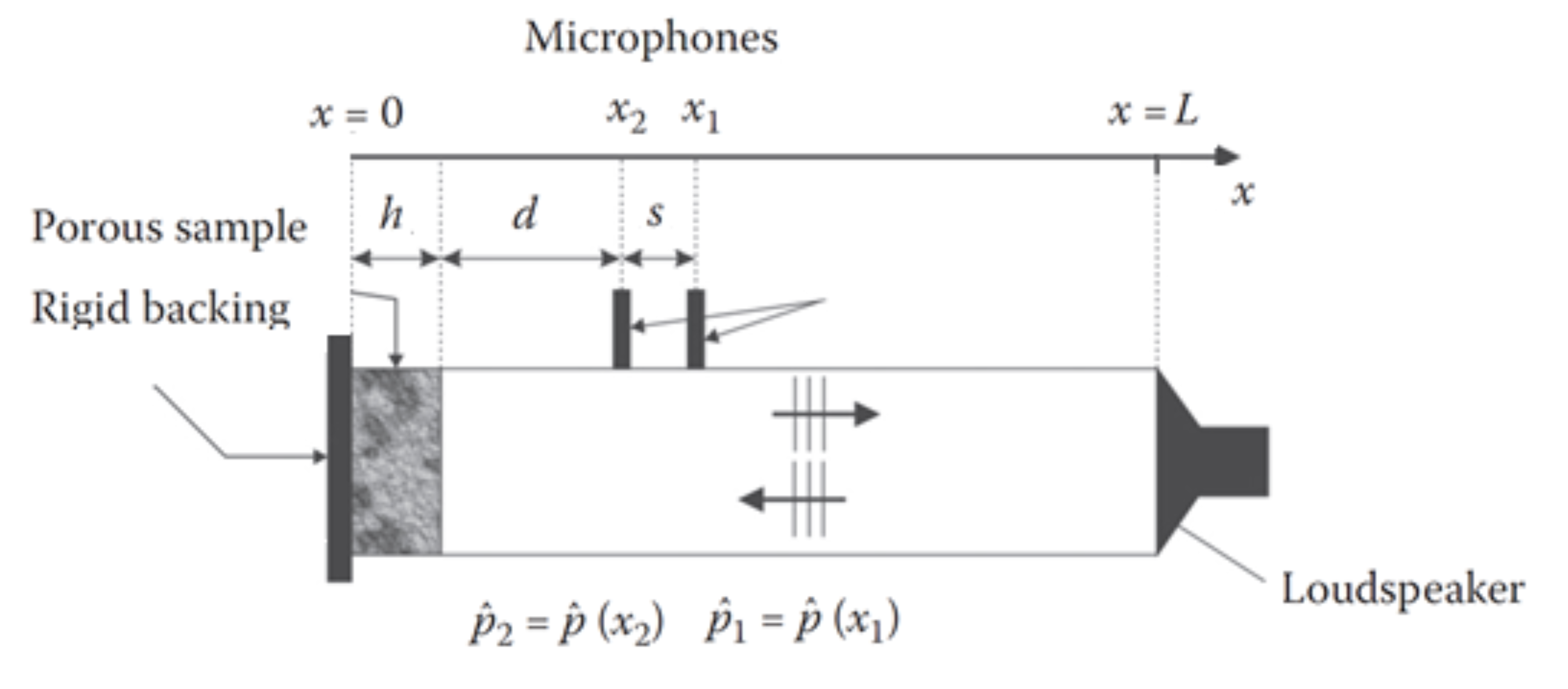
The impedance of a material of thickness \(h\) bonded onto a rigid wall (\(x=0\)) and excited by a plane wave with incidence angle \(\theta=0\) is given by (Allard and Atalla, 2009).
\[ \hat{Z} = -i\hat{Z}_c\cot(\hat{k}_ch). \]In the following the loudspeaker is modeled as a displacement of \(\bar{U}_n=1\). Furthermore, the specific details of the setup is described as
Diameter of impedance tube \(D = 10\) cm (and thus cut-off frequency \(\frac{0.59c_0}{D} \approx 2006\) Hz).
Length of impedance tube: \(L = 10D\).
Microphone spacing: \(s = \frac{1}{2}D\).
Distance between microphone 2 and the surface of the material: \(d=D/2\).
Thickness of the material: \(h = 2 \text{cm}\).
Characteristic impedance \(\hat{Z}_c = \rho_0c_0\left[1 + 0.057X^{-0.754} - i0.189X^{-0.732}\right]\) (where \(X = \frac{\rho_0 f}{\rho_p}\)).
Wave number \(\hat{k}_c = \frac{\omega}{c_0}\left[1 + 0.0978X^{-0.700} - i0.189X^{-0.595}\right]\) (where \(X = \frac{\rho_0 f}{\rho_p}\)).
Density and propagation speed: \(\rho_0 = 1.2\ \text{kg}\text{m}^3\), \(c_0 = 340\) m/s.
Flow resistivity of the material \(\rho_p = 10000\) Rayls/m.
Finite Element Modeling
A 1D model of an impedance tube with a loudspeaker at \(x=L\) and a material at \(x=0\) can be described by the following set of equations
\[ \begin{cases} \frac{\mathrm{d}^2p}{\mathrm{d}x^2}(x) + \left(\frac{\omega}{c}\right)^2p(x) = 0,\ x\in[0,L]\\ \frac{\mathrm{d}p}{\mathrm{d}n}(L) = \mathrm{i}\rho\omega v_L = \rho\omega^2U_L\\ \frac{\mathrm{d}p}{\mathrm{d}n}(0) = ik\beta p(0) = ik\beta p_1 \end{cases} \]The PDE can is modeled using the FEM as previously
\[ \left(\mathbf{K} - k^2\mathbf{M}\right)\mathbf{p} = \mathbf{0}. \]However, in this case \(\int_{\partial\Omega}\phi(x)\frac{\partial p}{\partial n}(x)\ \mathrm{d}\mathbf{x} \neq 0\). Instead we have that
\[ \begin{aligned} \left[\phi(x)\frac{\mathrm{d}p}{\mathrm{d}n}(x)\right]_0^L &= \mathbf{a}^\top\mathbf{T}(L)\frac{\mathrm{d}p}{\mathrm{d}x}(L) - \mathbf{a}^\top\mathbf{T}(0)\frac{\mathrm{d}p}{\mathrm{d}x}(0)\\ &= \mathbf{a}^\top\left(\begin{bmatrix}0 \\ 0 \\ \vdots \\ 1\end{bmatrix}\rho\omega^2U_L - \begin{bmatrix}1 \\ 0 \\ \vdots \\ 0\end{bmatrix}ik\beta p(0)\right)\\ &= \mathbf{a}^\top\left(\begin{bmatrix}0 \\ 0 \\ \vdots \\ 1\end{bmatrix}\rho\omega^2U_L - \text{diag}\left(\begin{bmatrix}ik\beta \\ 0 \\ \vdots \\ 0\end{bmatrix}\right)\mathbf{p}\right).\\ \end{aligned} \]Where in the above we utilized the prescribed boundary conditions as well as the definition of \(\mathbf{T}(x)\). Putting things together we find that
\[ \left(\mathbf{K} - k^2\mathbf{M}+ \text{diag}\left(\begin{bmatrix}ik\beta \\ 0 \\ \vdots \\ 0\end{bmatrix}\right)\right)\mathbf{p} = \begin{bmatrix}0 \\ 0 \\ \vdots \\ 1\end{bmatrix}\rho\omega^2U_L. \]Numerical Results
Using the previously implemented FEM routines we can numerically solve the problem. The analytical expression is used to check the results.
using Plots
## Recomputing FEM matrices
K,M = assembly3(Me,Ke,nnt,ne) # (using @btime earlier means not storing the results)
## Setup
ρ₀ = 1.2   # Fluid density
c₀ = 342.2 # Speed of sound
Uₙ = 1     # Piston displacement
D = 0.1    # Diameter of Impedance Tube
s = 0.5*D  # Microphone spacing
d = D/2    # Distance between mic 2 and sample
## Frequency domain
fc = floor(1.84*c₀/D/pi) # Cut off frequency
freq = Vector(100:2:fc)  # Choose correctly the lowest frequency ( a funtion of mics spacing)
ω = 2*pi*freq
k₀ = ω/c₀
## Impedance properties
Z₀ = ρ₀ * c₀
h = 0.02  # thickness of the material
σ = 10000 # flow resitivity
X = ρ₀*freq/σ
Zc = Z₀*(1 .+ 0.057*X.^(-0.754)-im*0.087.*X.^(-0.732))
k = k₀ .*(1 .+0.0978*X.^(-0.700)-im*0.189.*X.^(-0.595))
Z = -im.*Zc.*cot.(k*h) / Z₀
beta= 1.0 ./ Z # convert to admittance
# Finding nodes located on the microphones.
in2=findall(x->x,abs.(x .-d) .< 1e-6)[1]        # Location of mic 2
in1=findall(x->x,abs.(x .-(d+s)) .<1e-6)[1]     # Location of mic 1
# Correcting the s and d distances to fit the numerical values.
s=abs(x[in1] - x[in2])  # Recalculate microphones separation
d=x[in2]                # Recalculate the distance between microphone 2 and the sample

## Output
ndof = nnt
nfreqs = length(ω)
P_mic1 = zeros(ComplexF64,nfreqs)
P_mic2 = zeros(ComplexF64,nfreqs)
A = Diagonal(zeros(ComplexF64,nnt))
F = zeros(ComplexF64,ndof) # Initialize force vector
k = ω/c₀

## Frequency sweep
for i in eachindex(ω)
    A[1,1] = im*k[i]*beta[i]
    F[end,1] = ρ₀*ω[i]^2*Uₙ
    S = K - k[i]^2*M + A
    p = S\F
    P_mic2[i] = p[in2]
    P_mic1[i] = p[in1]
end

# Calculate the normalized impedance
H₁₂ = P_mic2./P_mic1
R = (H₁₂ - exp.(-im*k*s))./(exp.(im*k*s)-H₁₂) .*exp.(im*2*k * (d + s))
Z_num = (1 .+ R)./(1 .- R)
## Comparison with the exact solution
plot(freq,real.(Z),label="Analytical",linewidth=2)
plot!(freq,real.(Z_num),label="FEM",linestyle=:dash,linewidth=2)
xlims!((100, 2000))
xlabel!("Frequency (Hz)")
ylabel!("Normalized Impedance - Real part")
Example: Computing modes in 2D
The Finite Element Method can also be used to compute the modes, i.e. finding the eigenvalues of the system
\[ c^2\mathbf{K} - \omega^2\mathbf{M}. \]For a square room with side lengths \(L_x\) and \(L_y\) the modes can be computed analytically as
\[ \frac{c}{2}\sqrt{\left(\frac{n_x}{L_x}\right)^2 + \left(\frac{n_y}{L_y}\right)^2}. \]## Defining geometry.
Lx = 10
Ly = 4
n = 20+1
m = 8+1
ne = (n-1)*(m-1) # Number of linear elements
nnt = n*m # Total number of nodes
## Plotting the elements
x = Vector(0:Lx/(n-1):Lx)
y = Vector(0:Ly/(m-1):Ly)
X = kron(x,ones(m))
Y = kron(ones(n),y)
scatter(X,Y,aspect_ratio=1,legend=false,gridlinewidth=1,gridalpha=1,alpha=0,background=:gray,background_color_outside=:white)
xticks!(x); xlims!((0,Lx)); xlabel!("x");
yticks!(y); ylims!((0,Ly)); ylabel!("y");
The Finite Element computation for the 2D room will look similar to the one for the 1D impedance tube. However, one difference is the reliance on the topology/connectivity matrix. The code look as follows
## Creating the topology
T = reshape(1:nnt,m,n)      # Numbering all nodes on the grid
topology = zeros(Int,4,ne)  # Allocating the topology
topology[1,:] = T[1:end-1,1:end-1][:]   # Extracting submatrix
topology[2,:] = T[2:end,1:end-1][:]     # Extracting submatrix
topology[3,:] = T[2:end,2:end][:]       # Extracting submatrix
topology[4,:] = T[1:end-1,2:end][:]     # Extracting submatrix
## Computing Element matrices
# Defining local basis functions (and gradient using ForwardDiff - This is inefficient but easy)
Tᵉ(u)  = [(1-u[1])*(1-u[2]);(1+u[1])*(1-u[2]);(1+u[1])*(1+u[2]);(1-u[1])*(1+u[2])]'/4
∇Tᵉ(u) = hcat(ForwardDiff.jacobian(Tᵉ,u))'
# Every element is the same, so the Jacobian does not depend on the element in this case.
# Furthermore we map from [-1,1] onto [x_i,x_{i+1}]. Meaning from length 2 to length h.
jacobian(u) = (x[2]-x[1])/2*(y[2]-y[1])/2
# In the 1D case the Jacobian function and matrix are equal. This is not true in higher dimensions.
J(u) = Diagonal([x[2]-x[1];y[2]-y[1]])/2
# Defining the local element matrices. Since the elements are the same size its constant.
Q = 2  # Number of Gaussian points used in the integration.
u,wu = gausslegendre(Q)
v,wv = gausslegendre(Q)
U = kron(u,ones(Q))
V = kron(ones(Q),v)
W = kron(wu,wv)
P = [U';V']

Me = sum(i -> W[i]*jacobian(P[:,i])*Tᵉ(P[:,i])'*Tᵉ(P[:,i]),1:2Q)
Ke = sum(i -> W[i]*jacobian(P[:,i])*∇Tᵉ(P[:,i])'*J(P[:,i])^(-1)*J(P[:,i])^(-1)'*∇Tᵉ(P[:,i]),1:2Q)

## Assembly
function connected_topology(topology,nnt,ne)
    source_connections = [zeros(Int,0) for _ in 1:nnt]
    for element = 1:ne
        for i = 1:4
            append!(source_connections[topology[i,element]],topology[:,element])
        end
    end
    sort!.(unique.(source_connections))
end
function create_I_J(connections)
    I = zeros(Int,sum(length.(connections)))
    J = zeros(Int,sum(length.(connections)))
    lower = 1
    for (idx,con) in enumerate(connections)
        upper = lower + length(con)
        I[lower:upper-1] .= con
        J[lower:upper-1] .= idx
        lower = upper
    end
    return I,J
end
function assembly(Me,Ke,topology,nnt)
    ne = size(topology,2)
    connections = connected_topology(topology,nnt,ne)
    I,J = create_I_J(connections)
    S = sparse(I,J,1:length(I)) # Sparse matrix representing the indices of Kd and Md
    Kd = zeros(length(I))
    Md = zeros(length(I))
    for ie=1:ne
        top = topology[:,ie]
        Kd[S[top,top]] += Ke
        Md[S[top,top]] += Me
    end
    K = sparse(I,J,Kd)
    M = sparse(I,J,Md)
    return K,M
end
K,M = assembly(Me,Ke,topology,nnt);

using Arpack
F = eigs(c₀^2*K,M,which=:SM,nev=10);
freq = sort(sqrt.(abs.(F[1]))/2/π);
plot((contourf(x,y,reshape(F[2][:,id],m,n),linewidth=0,levels=1000,legend=false,axis=false,title="$(round(freq[id],digits=2)) Hz") for id in 2:10)..., layout = (3, 3)) 
This can be compared to the analytical eigenvalues computed by
nx, ny = 0:4, 0:4
freq_analytical = c₀/2*sqrt.((nx/Lx).^2 .+ (ny'/Ly).^2)
analytical_freqs = sort(freq_analytical[:])
print(round.(analytical_freqs[2:10],digits=2))
[17.11, 34.22, 42.78, 46.07, 51.33, 54.78, 66.82, 68.44, 80.71]